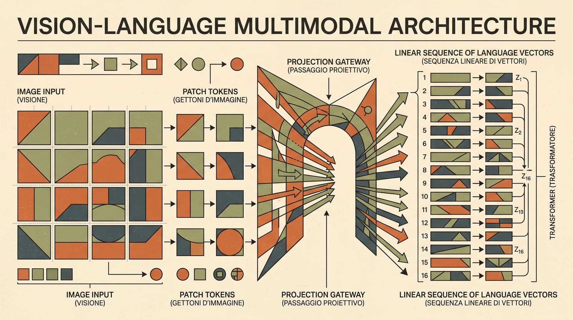
Vision-Language Model Architectures: How Vision Encoders, Token Projectors, and Dynamic Resolution Bridge Modalities

Modern large language models operate exclusively on discrete sequences of token embeddings. Integrating visual perception into these systems requires converting continuous, two-dimensional spatial arrays into linear sequences of embedding vectors that match the dimensionality and distribution of the language model's hidden states.

Vision-language models (VLMs) like LLaVA, Flamingo, Qwen2-VL, and InternVL accomplish this conversion through a three-stage pipeline: a vision encoder, a cross-modal projector, and a decoder-only language model backbone. Over recent architectural generations, the core engineering challenges have shifted from basic cross-modal alignment toward preserving fine-grained spatial resolution, managing token overhead, and optimizing inference-time memory consumption.

The Multimodal Embedding Formulation

An autoregressive language model processes a sequence of text tokens converted into dense vectors:

$\mathbf{H}_0 = [\mathbf{e}(t_1), \mathbf{e}(t_2), \dots, \mathbf{e}(t_L)] \in \mathbb{R}^{L \times d_{LLM}}$

To introduce an image $\mathbf{I} \in \mathbb{R}^{H \times W \times C}$ , the vision system transforms the image into a sequence of $N_v$ visual tokens:

$\mathbf{X}_v = [\mathbf{v}_1, \mathbf{v}_2, \dots, \mathbf{v}_{N_v}] \in \mathbb{R}^{N_v \times d_{LLM}}$

These visual tokens are prepended or interleaved with the text tokens to form a unified input sequence $\mathbf{H}_0 = [\mathbf{X}_v \,;\, \mathbf{X}_t]$ . The language model autoregressively generates subsequent text tokens using standard causal self-attention, treating visual tokens identically to text prefixes without requiring specialized multimodal attention layers during generation.

1. Vision Encoders: Patchification and Representation Space

The first stage extracts rich visual representations from raw pixel grids. Modern VLMs rely almost universally on Vision Transformers (ViT).

Patch Extraction

A Vision Transformer partitions an input image of height $H$ , width $W$ , and channels $C$ into non-overlapping spatial patches of size $P \times P$ (typically $14 \times 14$ or $16 \times 16$ pixels). The number of resulting patches is:

$N = \frac{H \cdot W}{P^2}$

Each patch is flattened into a vector of dimension $P^2 \cdot C$ and projected linearly to the vision encoder embedding dimension $d_{vision}$ . Learnable 1D or 2D positional embeddings are added to retain spatial orientation before passing through standard transformer encoder blocks.

Contrastive Pre-Training: CLIP vs. SigLIP

Vision encoders used in VLMs are rarely trained from scratch alongside the language model. Instead, they are pre-trained on web-scale image-text pairs:

CLIP (Contrastive Language-Image Pre-training): Radford et al. (2021) trained dual vision and text encoders using InfoNCE symmetric cross-entropy loss over batch similarities. InfoNCE normalizes similarities across all pairs in a batch, requiring large batch sizes ( $32\text{k}+$ ) and cross-device communication during distributed pre-training.
SigLIP (Sigmoid Loss for Language Image Pre-Training): Zhai et al. (2023) replaced the softmax-normalized loss with a pairwise sigmoid loss:

$\mathcal{L} = -\sum_{i=1}^B \sum_{j=1}^B \log \sigma \left( (-1)^{\mathbb{I}[i \neq j]} \cdot (t \cdot \mathbf{v}_i^\top \mathbf{u}_j + b) \right)$

SigLIP treats each image-text pair as an independent binary classification problem. By eliminating the global softmax normalization denominator, SigLIP removes cross-GPU all-gather communication bottlenecks, performs stably at smaller batch sizes, and yields higher semantic retrieval accuracy. As a result, SigLIP-SO400M and SigLIP-2 have largely superseded original OpenAI CLIP checkpoints as the default vision backbones in open-weight models.

Feature Selection and Layer Pooling

Standard contrastive training encourages the final layer of a vision encoder to discard localized spatial details in favor of global semantic classification. To preserve spatial precision necessary for object grounding and optical character recognition (OCR), architectures like LLaVA extract feature activations from the penultimate layer (e.g., layer $-2$ ) of the vision backbone instead of the final classification layer.

VLM Projector and Dynamic Tiling Architectures

The visual feature dimension $d_{vision}$ rarely matches the language model's hidden dimension $d_{LLM}$ (for example, SigLIP-SO400M outputs $d_{vision} = 1152$ , while a 7B LLM requires $d_{LLM} = 4096$ ). The cross-modal projector translates visual tokens into the language representation space.

Three main projector paradigms dominate the literature:

Linear and MLP Projectors

Introduced in early LLaVA models and refined in LLaVA-1.5, this approach uses a simple multi-layer perceptron with non-linear activation:

$\mathbf{X}_v = \mathbf{W}_2 \cdot \text{GELU}(\mathbf{W}_1 \mathbf{Z}_v + \mathbf{b}_1) + \mathbf{b}_2$

Advantages: Minimal parameter overhead (typically 10M to 50M parameters), fast convergence, and no architectural information bottleneck. Every visual patch is preserved as an individual token.
Disadvantages: Token count scales linearly with patch count. A single $336 \times 336$ image with $14 \times 14$ patches generates $24 \times 24 = 576$ visual tokens, creating significant memory overhead in multi-image or video contexts.

Perceiver Resamplers and Q-Formers

Pioneered by Flamingo and BLIP-2, this architecture uses a fixed set of $K$ learnable query embeddings (e.g., $K = 32$ or $64$ ) that attend to the variable-length visual features $\mathbf{Z}_v$ via cross-attention layers.

Advantages: Fixed output token budget regardless of input image size, dramatically reducing LLM prompt length and key-value (KV) cache memory.
Disadvantages: Lossy compression. Compressing hundreds of patch representations into 32 or 64 fixed slots discards fine spatial details, degrading performance on document understanding, dense OCR, and small-object detection.

Spatial Downsampling and Pixel Unshuffle

Modern models such as Qwen2-VL and InternVL combine spatial inductive biases with token reduction by grouping adjacent $2 \times 2$ patch tokens:

$\mathbf{z}_{\text{merged}} = [\mathbf{z}_{2i, 2j} \,;\, \mathbf{z}_{2i+1, 2j} \,;\, \mathbf{z}_{2i, 2j+1} \,;\, \mathbf{z}_{2i+1, 2j+1}]$

The concatenated vectors are then linearly projected from $4 \cdot d_{vision}$ to $d_{LLM}$ . This spatial pooling reduces token counts by 75% ( $576 \to 144$ tokens per tile) while maintaining explicit 2D relative coordinate structures.

3. Dynamic High-Resolution Tiling and Aspect Ratio Handling

Standard Vision Transformers require fixed-size, square input images (such as $224 \times 224$ or $336 \times 336$ pixels). Resizing high-resolution or non-square images to fixed squares introduces two critical failure modes:

Aspect Ratio Distortion: Anamorphic scaling stretches or compresses text and visual features, distorting geometry.
Sub-Sampling Blur: Downsampling a $4000 \times 3000$ document image to $336 \times 336$ destroys high-frequency details, rendering small text unreadable.

Two primary techniques resolve these limitations:

AnyRes Dynamic Tiling

Used in LLaVA-NeXT, SPHINX, and InternVL, AnyRes segments arbitrary-resolution images into grids of standard-sized tiles alongside a low-resolution thumbnail:

Calculate the optimal grid configuration (e.g., $1 \times 2$ , $2 \times 2$ , $1 \times 3$ ) that matches the original aspect ratio with minimal padding.
Crop the image into $M$ local patches of size $P_{res} \times P_{res}$ , plus one global downsampled overview image.
Pass all $M + 1$ crops through the vision encoder independently.
Insert special separator tokens (such as \n row delimiters) between patch rows to preserve 2D topological layout before passing the flattened sequence to the LLM.

Native Dynamic Resolution and 3D Rotary Position Embeddings

NaViT and Qwen2-VL eliminated fixed grid cropping by introducing native sequence packing and Multimodal Rotary Position Embeddings (M-RoPE).

Instead of forcing images into square grids, Qwen2-VL processes variable numbers of patches directly without padding. To track spatial and temporal coordinates across mixed text, image, and video inputs, M-RoPE decomposes rotary positional embeddings across three dimensions:

Temporal ID ( $t$ ): Tracking frame index in video or sequential inputs.
Height ID ( $h$ ): Tracking vertical patch coordinates.
Width ID ( $w$ ): Tracking horizontal patch coordinates.

For pure text tokens, $t = h = w = \text{pos}$ . For 2D image patches, $t$ is constant while $h$ and $w$ encode spatial grid offsets. This approach allows the attention mechanism to compute true 2D spatial distances directly in the rotational query-key dot products.

4. The Two-Stage Training Paradigm

Training vision-language models from scratch end-to-end is computationally prohibitive. Modern VLMs rely on a decoupled two-stage recipe:

Stage 1: Feature Alignment
[Image] -> [Vision Encoder (Frozen)] -> [Projector (Trainable)] -> [LLM (Frozen)] -> Loss
Target: Align vision embeddings with text token distribution using captioning data.

Stage 2: Visual Instruction Tuning
[Image] -> [Vision Encoder (Frozen/Unfrozen)] -> [Projector (Trainable)] -> [LLM (Unfrozen)] -> Loss
Target: Multi-turn reasoning, OCR, grounding, and instruction following.

Stage 1: Feature Alignment

Objective: Teach the projector to translate visual features into the LLM's pre-existing token embedding manifold.
Weights: The vision encoder and LLM backbone remain completely frozen; only the projector weights are updated.
Dataset: Hundreds of thousands to millions of synthetic image-caption pairs (such as filtered CC3M or LAION subsets).

Stage 2: Visual Instruction Tuning

Objective: Train the system to follow multi-modal instructions, execute visual reasoning, and parse complex documents.
Weights: The projector is fully updated. The LLM backbone is either fine-tuned with parameter-efficient methods (LoRA) or fully unfrozen. In advanced configurations (such as InternVL-2.5), the vision encoder is also unfrozen with a reduced learning rate.
Dataset: Diverse instruction-response pairs covering conversational visual QA, document OCR, chart analysis, geometric reasoning, and bounding-box coordinate prediction.

5. Serving Bottlenecks: Memory and TTFT

Deploying VLMs in production reveals severe latency and throughput trade-offs compared to text-only language models:

Time To First Token (TTFT) Inflation: A single high-resolution image processed via dynamic tiling can produce 2,000 to 4,000 visual tokens. In multi-turn chat, re-evaluating long visual prefixes across every conversational turn creates massive prefill computation bottlenecks.
Key-Value (KV) Cache Growth: In standard decoder-only serving engines, every visual prefix token consumes dedicated memory in the paged KV cache for the entire lifetime of the request. A 32-layer model with Grouped-Query Attention (16 KV heads, head dimension 128) consumes approximately 1.05 MB per 1,000 tokens in FP16. Multi-image document pipelines rapidly exhaust GPU memory bandwidth.
Visual Token Eviction: To mitigate these serving costs, modern inference runtimes are increasingly implementing visual token compression techniques, such as pruning redundant background patches via spatial attention masks or caching static visual KV states across multi-turn sessions.

Vision-Language Model Architectures: How Vision Encoders, Token Projectors, and Dynamic Resolution Bridge Modalities

The Multimodal Embedding Formulation