
Information retrieval systems in production Retrieval-Augmented Generation (RAG) and enterprise search have transitioned through multiple reranking paradigms. While first-stage retrieval (dense vector embeddings and sparse lexical BM25/SPLADE) retrieves candidate sets of 50 to 200 documents in under 20 milliseconds, the precision of downstream generation depends heavily on the reranking stage.
Traditional neural rerankers evaluate candidates through pointwise scoring or pairwise classification. However, the emergence of listwise large language model rerankers, spearheaded by RankGPT (Sun et al., 2023) and distilled open-weight models like RankVicuna (Pradeep et al., 2023) and RankZephyr (Pradeep et al., 2023), has introduced a fundamentally different serving dynamic. Rather than scoring documents in isolation, listwise architectures evaluate candidate sets collectively inside an autoregressive context window.
Understanding the architectural mechanics, positional biases, sliding-window algorithms, and token economics of listwise reranking is essential for engineering low-latency, high-precision retrieval pipelines.

The Reranking Hierarchy: Pointwise, Pairwise, and Listwise
Neural rerankers operate across three distinct structural formulations:
1. Pointwise Scoring
Pointwise architectures (such as monoBERT, monoT5, and standard BGE cross-encoders) take a query and a single document, outputting an independent scalar relevance probability.
- Computational Complexity: O(N) forward passes for N candidate documents.
- Serving Strengths: Embarrassingly parallelizable across GPU workers, predictable latency, and per-document score cacheability.
- Architectural Limitations: Inability to perform cross-document comparison. A pointwise model evaluates each document in a vacuum, preventing it from detecting mutual redundancy, complementary facts across passages, or relative topical depth.
2. Pairwise Comparison
Pairwise architectures (such as duoBERT and Pairwise Ranking Prompting) evaluate document pairs to determine the relative preference probability between two passages.
- Computational Complexity: O(N^2) comparisons for full tournament ranking, or O(N log N) using sorting networks.
- Serving Strengths: Directly optimizes relative order rather than absolute score calibration.
- Architectural Limitations: Massive computational overhead for candidate sets above 20 items, and vulnerability to Condorcet cycles where non-transitive preferences break sorting invariants.
3. Listwise LLM Reranking
Listwise architectures present the query alongside an ordered sequence of candidate passages identified by token tags (for example, [1], [2], [3]). The language model is prompted to generate the sorted permutation directly:
Rank the following 10 passages based on relevance to the query.
Query: {query}
[1] Passage A content...
[2] Passage B content...
...
[10] Passage J content...

Output the ranking as: [3] > [1] > [10] > ...- Computational Complexity: Single LLM invocation per window, scaling linearly with candidate size via sliding windows.
- Serving Strengths: Full cross-document self-attention allows the transformer layers to weigh passage credibility, eliminate near-duplicate passages, and evaluate relative completeness.
- Architectural Limitations: Context length ceilings, high input token consumption, and autoregressive generation latency.
The Sliding-Window Bubble-Sort Algorithm
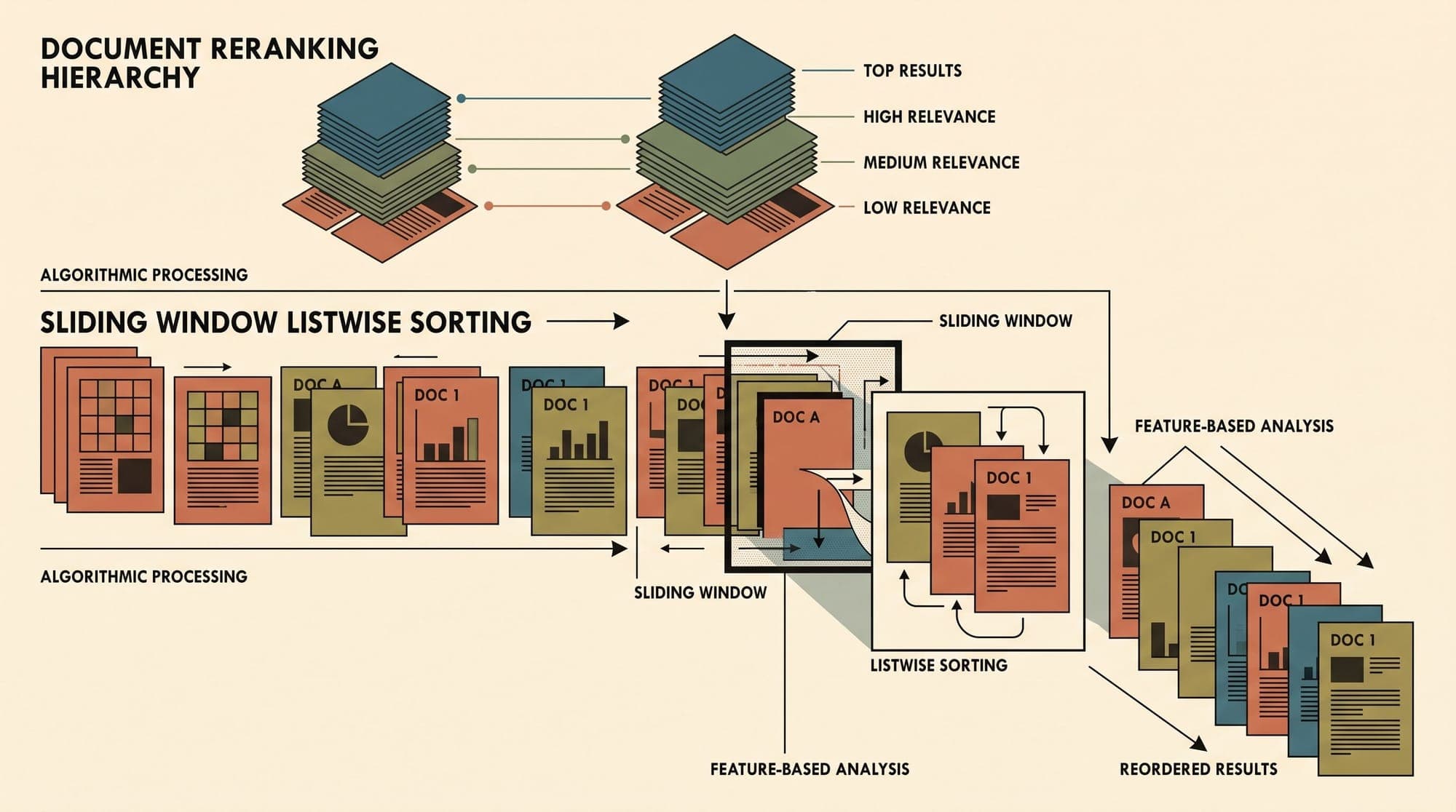
Standard context windows and generative attention budgets prevent feeding 100 long passages into a single listwise prompt. To scale listwise reranking to deep candidate pools (such as N = 100), Sun et al. (2023) established the sliding-window permutation protocol.
The algorithm mirrors a bubble-sort pass from the bottom of the candidate list to the top:
- Window Sizing and Stride: Define a window capacity (typically 20 passages) and a stride step (typically 10 passages).
- Bottom-Up Traversal: The first iteration ingests the lowest-ranked window. The model evaluates the 20 items and generates their internal permutation.
- Candidate Promotion: The top 10 candidates from the newly sorted window are swapped upward into the next overlapping window.
- Iterative Passes: The sliding window shifts toward the head of the list until reaching index 0.
For a candidate list of 100 documents with a window size of 20 and a stride of 10, the total number of sequential LLM inference steps is exactly 9 calls.
This sliding bubble-sort ensures that any high-relevance document mistakenly ranked near the bottom by first-stage retrieval can bubble up to the top rank across multiple window iterations.
Mitigating Positional Bias: Permutation Self-Consistency
Large language models suffer from pronounced positional biases. Research by Tang et al. (2023) demonstrated that listwise rerankers exhibit substantial primacy and recency biases, frequently favoring passages placed at the beginning or end of the prompt regardless of relevance.
To enforce order-invariance, Tang et al. introduced Permutation Self-Consistency (PSC):
- Stochastic Permutation Sampling: Given an input candidate list, create M randomly shuffled input permutations.
- Parallel Inference: Prompt the listwise LLM concurrently across all M permutations to generate M output rankings.
- Kendall Tau Consensus Aggregation: Aggregate the output rankings into a unified consensus permutation that minimizes the average Kendall tau distance across all generated outputs.
Empirical evaluation on TREC Deep Learning benchmarks reveals that Permutation Self-Consistency boosts nDCG@10 by 2 to 4 points while eliminating sensitivity to the initial retriever ordering.
Open-Weight Distillation: RankVicuna and RankZephyr
Relying on proprietary commercial APIs (such as GPT-4) for 9 sequential sliding-window calls per search query introduces unviable latency (2,000 to 5,000 milliseconds) and high per-query costs.
To solve this, researchers distilled listwise ranking capabilities into compact 7B-parameter open-weight models:
- RankVicuna: Fine-tuned Vicuna-7B/13B on RankGPT-3.5 permutation trajectories using hard rank-loss supervision.
- RankZephyr: Fine-tuned Zephyr-7B-beta on high-quality RankGPT-4 distillation data across BM25 and SPLADE++ retrieval splits.
On the TREC Deep Learning 2019 (DL19) and 2020 (DL20) benchmarks, RankZephyr achieves an nDCG@10 of 0.7816 on DL19 and 0.7598 on DL20 when paired with SPLADE++ first-stage retrieval, matching or outperforming zero-shot RankGPT-4 while running locally on a single GPU.
Production Cascading Architecture and Serving Economics
Deploying listwise rerankers in production requires a multi-tier cascade to balance latency budgets and token costs:
- Tier 1: Candidate Selection (Vector Index / BM25 / SPLADE): Prunes 10,000,000 records to the top 100 candidates in 10 to 25 milliseconds.
- Tier 2: High-Throughput Pointwise Pruning (Cross-Encoder / ColBERT): Evaluates the 100 candidates and selects the top 20 in 15 to 35 milliseconds.
- Tier 3: Listwise Permutation Ranking (RankZephyr / Single-Window SLM): Reranks the top 20 candidates into final top-5 generation context in 80 to 160 milliseconds.
Token Economics and Latency Breakdown
Evaluating a single window of 20 documents with an average passage length of 150 tokens:
- Prompt Input Tokens: (20 documents * 150 tokens) + 100 instruction tokens = approximately 3,100 tokens.
- Generation Output Tokens: 20 rank identifiers = approximately 40 tokens.
In an inference engine with prefix caching and FlashAttention-2, time-to-first-token (TTFT) for a 3,100-token prefill on an NVIDIA H100 GPU is approximately 25 milliseconds, while autoregressive decoding of 40 tokens requires roughly 40 milliseconds.
By filtering down to 20 candidates in Tier 2, production systems eliminate the need for multi-step sliding-window bubble sorting during Tier 3, executing a single 20-candidate listwise pass in under 100 milliseconds total latency.
Sources
- Sun, W., et al. (2023). Is ChatGPT Good at Search? Investigating Large Language Models as Re-Ranking Agents. arXiv:2304.09542.
- Pradeep, R., Sharifymoghaddam, S., & Lin, J. (2023). RankVicuna: Zero-Shot Listwise Document Reranking with Open-Source Large Language Models. arXiv:2309.15088.
- Pradeep, R., Sharifymoghaddam, S., & Lin, J. (2023). RankZephyr: Effective and Robust Zero-Shot Listwise Reranking is a Breeze!. arXiv:2312.02724.
- Tang, R., Zhang, X., Ma, X., Lin, J., & Ture, F. (2023). Found in the Middle: Permutation Self-Consistency Improves Listwise Ranking in Large Language Models. NAACL 2024 / arXiv:2310.07712.



