
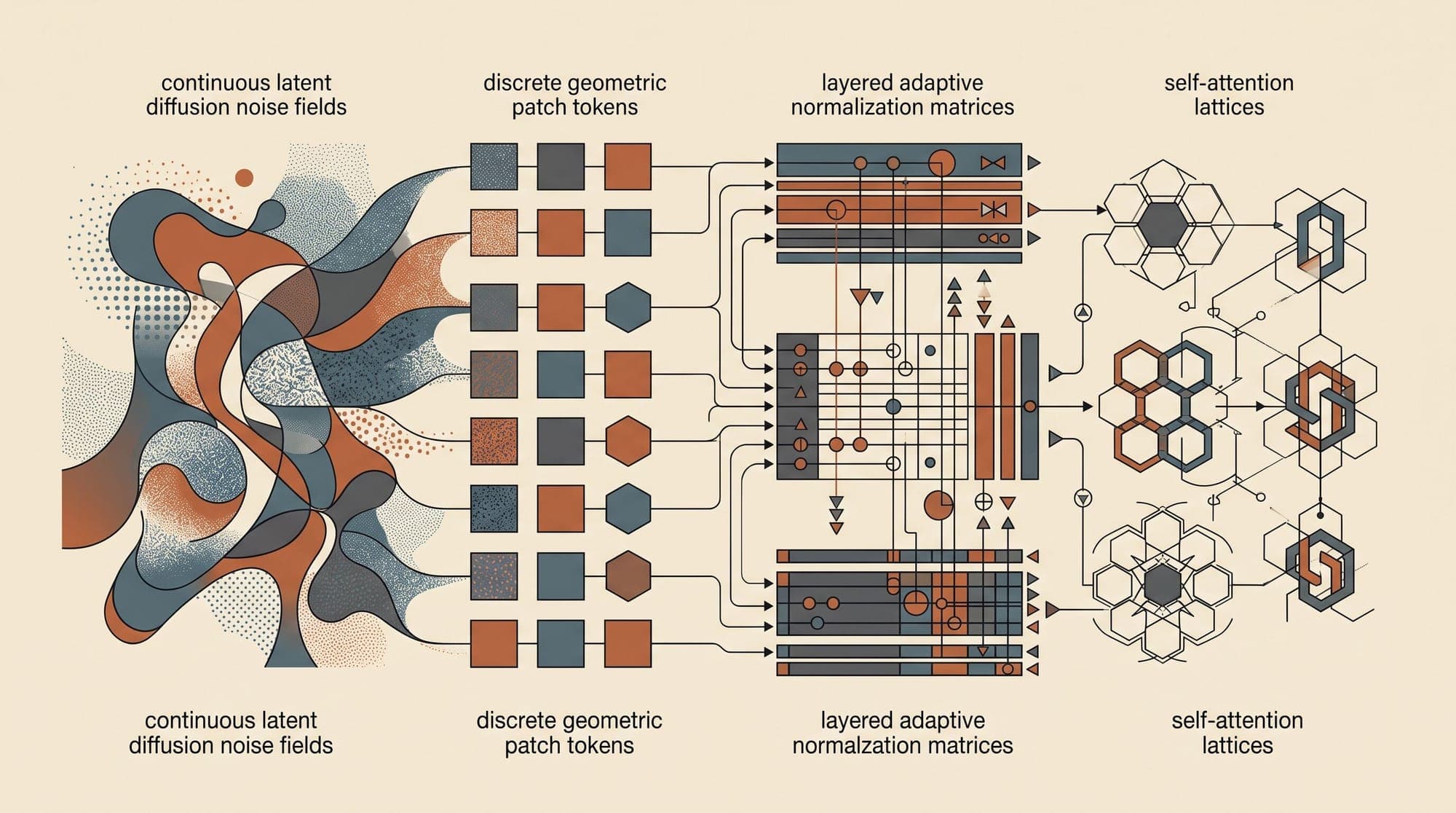
Diffusion Transformers (DiT), introduced by William Peebles and Saining Xie in their 2023 paper Scalable Diffusion Models with Transformers, established a structural departure in generative visual modeling. For years, diffusion pipelines relied almost exclusively on convolutional U-Net backbones derived from Denoising Diffusion Probabilistic Models (DDPM) and Latent Diffusion Models (LDM). DiT replaced these multi-scale convolutional networks with standard isotropic Transformer architectures operating on patchified latent tokens.
The design demonstrated that the power-law compute scaling observed in autoregressive language models transfers directly to diffusion-based generative tasks. Modern state-of-the-art text-to-image and text-to-video systems, including Stable Diffusion 3, FLUX.1, and OpenAI Sora, trace their core generative backbones directly to the Diffusion Transformer formulation.
The Architectural Shift: Replacing U-Nets with Transformers
Convolutional U-Nets process representations across downsampling and upsampling paths connected by skip connections. While effective for capturing local pixel correlations, U-Net architectures introduce spatial inductive biases that limit homogeneous hardware scaling and cross-modal parameter sharing.
DiT eliminates downsampling bottlenecks, residual down/up blocks, and convolutional operations entirely. Instead, the model processes latent tensors as sequences of flattened token embeddings through repeated Transformer blocks composed of multi-head self-attention and pointwise feedforward layers.
Latent Space Tokenization and Patchification
Operating transformers directly on high-resolution pixel space carries prohibitive computational complexity because self-attention scales quadratically with sequence length:
O(T^2)
To maintain computational efficiency, DiT operates within the continuous latent space of a pre-trained Variational Autoencoder (VAE). Given an RGB image input of dimensions:
x in R^(3 x H_img x W_img)
A pre-trained VAE encoder compresses the image by a spatial downsampling factor (typically f = 8), yielding a latent representation:
z = E(x) in R^(C x H x W)
For a standard 256x256 image with f = 8 and latent channel depth C = 4, the latent tensor has dimensions 4 x 32 x 32.
Spatial Patch Extraction
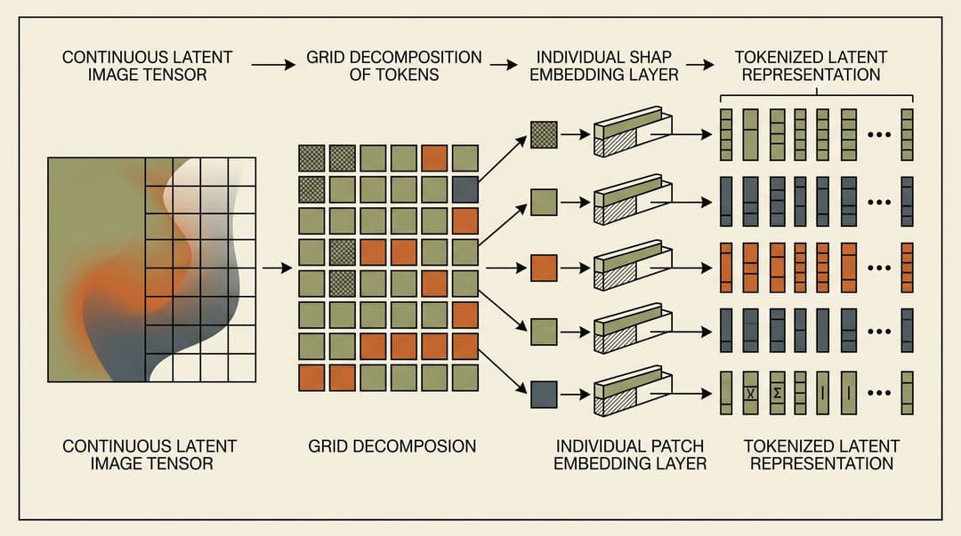
DiT converts the spatial latent tensor into a discrete sequence of tokens through patchification. Given a spatial patch dimension p:
- The latent grid is segmented into non-overlapping patches of size p x p x C.
- The total sequence length of tokens is T = (H / p) * (W / p).
- Each individual patch is flattened into a vector of dimension d = p^2 * C.
For a latent of size 32 x 32 with patch size p = 2, the sequence length is:
T = (32 / 2) * (32 / 2) = 16 * 16 = 256 tokens
Each patch vector is projected into the Transformer hidden dimension D via a learnable linear projection weight matrix W_emb in R^(d x D):
x_0 = [Flatten(patch_1) W_emb, Flatten(patch_2) W_emb, ..., Flatten(patch_T) W_emb]
Standard fixed 2D sinusoidal positional encodings are added to x_0 before the first Transformer layer to preserve spatial coordinate geometry.
Conditioning Mechanisms and adaLN-Zero
Diffusion models require conditioning signals to guide the reverse denoising trajectory. In class-conditional or text-conditional generation, the model receives a continuous diffusion timestep t and conditioning context y (such as a class label embedding or text representation).
Peebles and Xie evaluated four distinct conditioning strategies for Transformer backbones:
- In-Context Conditioning: Concatenating conditioning embeddings as additional prefix tokens in the input sequence.
- Cross-Attention: Injecting conditioning representations through dedicated multi-head cross-attention layers after self-attention.
- Adaptive Layer Normalization (adaLN): Regressing dimension-wise scale and shift parameters directly from conditioning embeddings.
- Adaptive Layer Normalization with Zero-Initialization (adaLN-Zero): Regressing scale, shift, and dimension-wise residual gating parameters while initializing gating layers to zero.
Empirical evaluations showed that adaLN-Zero achieved lower Fréchet Inception Distance (FID) than cross-attention and in-context conditioning while requiring fewer floating-point operations.
Mathematical Formulation of adaLN-Zero
In standard Layer Normalization, an input vector x is normalized to zero mean and unit variance, then modulated by learned static scale and shift parameters:
LayerNorm(x) = ((x - mu) / sigma) * gamma_static + beta_static
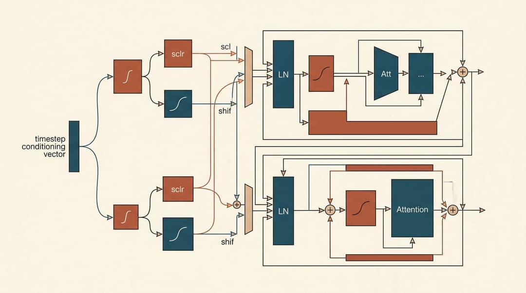
Under adaLN-Zero, static parameters are replaced by dynamically computed modulation vectors regressed from the conditioning embedding c = Embed(t) + Embed(y). A shared Multi-Layer Perceptron outputs six modulation vectors per Transformer block:
(gamma_1, beta_1, alpha_1, gamma_2, beta_2, alpha_2) = MLP(c)
The Transformer block applies these vectors across the multi-head self-attention (MSA) and pointwise feedforward (MLP) sub-layers:
- Modulated Self-Attention Sub-Layer:
h = x + alpha_1 * MSA((1 + gamma_1) * LayerNorm(x) + beta_1)
- Modulated Feedforward Sub-Layer:
y_out = h + alpha_2 * MLP((1 + gamma_2) * LayerNorm(h) + beta_2)
Where * denotes element-wise multiplication (Hadamard product).
Zero-Initialization Dynamics
The critical distinction in adaLN-Zero lies in its initialization scheme. The final linear projection layer of the conditioning MLP is initialized with all zeros.
At training step 0:
- gamma_1 = 0, beta_1 = 0, alpha_1 = 0
- gamma_2 = 0, beta_2 = 0, alpha_2 = 0
Because alpha_1 = 0 and alpha_2 = 0, the residual branches evaluate to zero, and the block reduces to an exact identity function:
h = x + 0 = x y_out = h + 0 = x
Similar to identity-mapping initializations in deep Residual Networks, zero-initialization ensures that gradient signals propagate uninhibited through arbitrary network depths at the start of training. This eliminates vanishing and exploding gradients without requiring complex warmup schedules.
Latent Diffusion Scaling Laws
A central contribution of the DiT architecture was formalizing compute scaling in diffusion models. Peebles and Xie configured four model scales:
- DiT-S (Small): 12 layers, hidden size 384, 6 attention heads, 33 million parameters
- DiT-B (Base): 12 layers, hidden size 768, 12 attention heads, 130 million parameters
- DiT-L (Large): 24 layers, hidden size 1024, 16 attention heads, 458 million parameters
- DiT-XL (Extra-Large): 28 layers, hidden size 1152, 16 attention heads, 675 million parameters
Each configuration was evaluated across patch sizes p in {8, 4, 2}. Decreasing patch size increases sequence length T by a factor of 4 for every halving of p, substantially raising total GigaFLOPs per forward pass.
Compute vs. Sample Quality Scaling
Across extensive training runs on ImageNet 256x256, Peebles and Xie identified consistent scaling patterns:
- Model Capacity and Token Resolution: Increasing Transformer parameter count (DiT-S to DiT-XL) and increasing sequence resolution (p=8 to p=2) monotonically reduced FID.
- GigaFLOPs Correlation: Total compute allocation (measured as model GigaFLOPs multiplied by training iterations) demonstrated a strong inverse power-law correlation with FID.
- Compute Efficiency: Scaling patch resolution (e.g., moving from DiT-XL/4 to DiT-XL/2) yielded steeper FID reductions per compute step than scaling model parameters at coarse patch resolutions.
DiT-XL/2 achieved a state-of-the-art FID of 2.27 on class-conditional ImageNet 256x256 (reaching 1.44 with classifier-free guidance), outperforming prior convolutional architectures including ADM (2.92) and LDM (3.60).
Architectural Evolutions in Production Systems
The basic DiT formulation has served as the baseline for modern generative diffusion systems, prompting several key architectural evolutions:
- Multimodal Diffusion Transformers (MMDiT): Introduced in Stable Diffusion 3, MMDiT maintains two separate sets of transformer weights for text embeddings and image latent tokens. Representations are processed independently through modality-specific self-attention before joining for shared attention layers.
- Joint Flow Matching Architectures: Modern systems such as FLUX.1 replace standard DDPM epsilon-prediction objectives with Rectified Flow Matching, integrating 2D Rotary Position Embeddings (RoPE) and combined single/double stream transformer blocks.
- Spatio-Temporal Patchification: Video generation models such as OpenAI Sora generalize 2D spatial patches into 3D spacetime volumes (p_time x p_height x p_width), enabling a single unified DiT architecture to train over variable-resolution images and videos.
Sources
- Scalable Diffusion Models with Transformers (Peebles & Xie, ICCV 2023)
- Denoising Diffusion Probabilistic Models (Ho et al., NeurIPS 2020)
- High-Resolution Image Synthesis with Latent Diffusion Models (Rombach et al., CVPR 2022)
- Scaling Rectified Flow Transformers for High-Resolution Image Synthesis (Esser et al., 2024)
- Black Forest Labs: Announcing FLUX.1 (2024)
- OpenAI: Video generation models as world simulators (2024)
