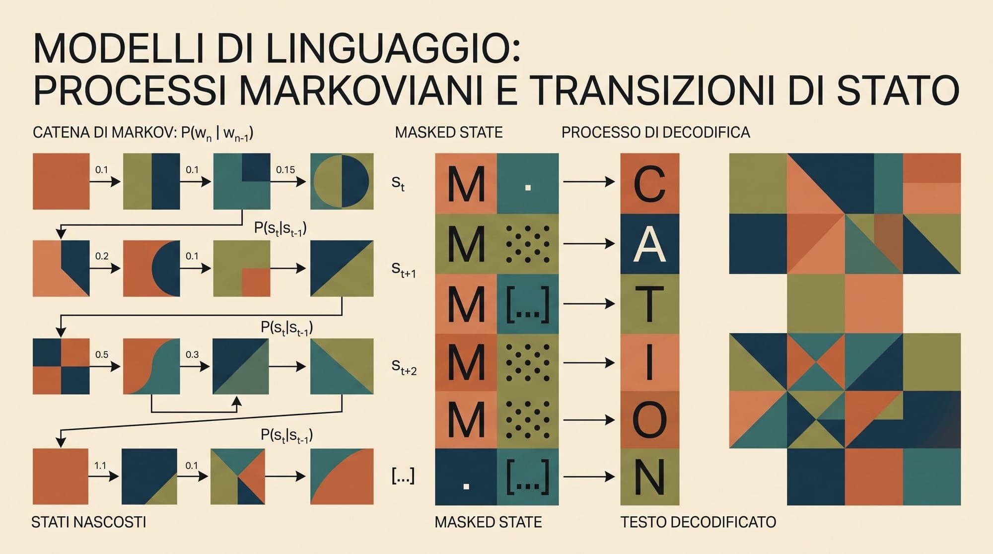
Discrete Diffusion in Large Language Models: How Continuous-Time Markov Chains, Absorbing States, and Score Entropy Challenge Autoregressive Generation

The dominance of autoregressive architectures in large language models rests on a fundamental mathematical formulation: the chain rule of probability. By factoring the joint distribution of a sequence into a product of conditional probabilities, $p(x) = \prod_{i=1}^N p(x_i \mid x_{<i})$ , autoregressive models reduce text generation to sequential next-token prediction.

While this left-to-right causal factorization has scaled effectively across compute regimes, it imposes rigid operational constraints. Autoregressive inference requires loading hundreds of billions of model parameters from high-bandwidth memory (HBM) to on-chip SRAM for every single generated token. This sequential memory-bound bottleneck caps decoding throughput. Furthermore, causal masking prevents native bidirectional context during generation, rendering infilling, span revision, and non-sequential editing inefficient.

Discrete diffusion language models have emerged as a mathematically grounded alternative. By modeling language generation not as a sequence of discrete choices, but as a continuous-time denoising trajectory over discrete state spaces, discrete diffusion decouples sequence length from generation steps and enables native bidirectional editing.

Discrete Diffusion Architecture and Forward-Reverse Markov Chain

Continuous Diffusion vs. The Categorical Bottleneck

Diffusion models originally gained prominence in continuous domains like image and audio generation, where corruption is governed by continuous stochastic differential equations (SDEs) of the form:

dx_t = f(x_t, t) dt + g(t) dw_t

In continuous spaces, score-based generative modeling relies on estimating the score function, $\nabla_x \log p_t(x)$ , which indicates the gradient of the log probability density with respect to spatial coordinates.

Applying this framework directly to text encounters immediate mathematical obstacles:

Lack of Continuous Geometry: Language tokens belong to a discrete categorical vocabulary $V = \{1, 2, \dots, K\}$ , typically numbering between 32,000 and 128,000 distinct tokens. There is no natural spatial gradient $\nabla_x$ in a discrete coordinate system.
Off-Manifold Rounding Errors: Early continuous-embedding diffusion methods (such as Diffusion-LM) projected discrete tokens into continuous embedding spaces, diffused Gaussian noise, and clamped the final vectors back to the nearest vocabulary embedding. This approach suffers from severe rounding errors, representation collapse, and poor likelihood bounds because the intermediate Gaussian trajectories traverse empty regions of the embedding manifold.

To model discrete text distributions rigorously, generative diffusion must operate directly over discrete state spaces using continuous-time Markov chains.

Continuous-Time Markov Chains on Discrete Vocabularies

In discrete diffusion, corruption is formalized as a Continuous-Time Markov Chain (CTMC) over the vocabulary $V$ . The transition dynamics are governed by a time-dependent transition rate matrix $Q_t \in \mathbb{R}^{K \times K}$ , where entry $Q_t(i, j)$ specifies the instantaneous probability per unit time that token $i$ transitions to token $j$ .

The forward transition probability over an infinitesimal time step $dt$ is defined as:

P(x_{t+dt} = j | x_t = i) = delta_{ij} + Q_t(i, j) dt + o(dt)

where $\delta_{ij}$ is the Kronecker delta, and the diagonal elements satisfy $Q_t(i, i) = -\sum_{j \neq i} Q_t(i, j)$ to ensure conservation of probability.

The probability distribution vector $p_t \in \mathbb{R}^K$ evolves according to the Master equation (Kolmogorov forward equation):

d p_t / dt = p_t Q_t

Given an initial clean text token $x_0$ , the conditional probability distribution at arbitrary forward time $t$ has the closed-form matrix exponential solution:

q(x_t | x_0) = x_0 exp( \int_0^t Q_s ds )

Transition Topologies: Uniform Noise vs. Absorbing States

The design of the rate matrix $Q_t$ defines how information is corrupted during the forward process. As established by Austin et al. in D3PM (Structured Denoising Diffusion Models in Discrete State-Spaces), two primary transition topologies dominate discrete diffusion:

1. Uniform Replacement (Categorical Corruption)

In uniform diffusion, any token can transition to any other token in the vocabulary with equal probability:

Q_t(i, j) = beta(t) / K   (for j != i)

As $t \to \infty$ , the forward marginal converges to a uniform distribution over the entire vocabulary: $q(x_\infty) \sim \text{Uniform}(V)$ . While theoretically symmetric, uniform noise suffers in large vocabularies ( $K \ge 32,000$ ). Replacing a token with a random vocabulary entry produces nonsensical sequences where the model cannot distinguish whether a token is original data or corrupt noise, diluting the training signal.

2. Absorbing State Diffusion (Masking)

In absorbing state diffusion, the vocabulary is expanded by a single absorbing state, denoted as the $[MASK]$ token: $\tilde{V} = V \cup \{[MASK]\}$ .

A token $x \in V$ transitions exclusively to $[MASK]$ with rate $\beta(t)$ , and the $[MASK]$ token has a zero exit rate (it is an absorbing state):

Q_t(i, [MASK]) = beta(t)   (for i in V)
Q_t(i, j) = 0              (for j != i, j in V)
Q_t([MASK], j) = 0         (for all j)

The forward marginal distribution $q(x_t \mid x_0)$ at time $t$ admits a simple closed form:

q(x_t | x_0) = alpha_t * delta(x_0) + (1 - alpha_t) * delta([MASK])

where $\alpha_t = \exp(-\int_0^t \beta(s)ds) \in [0, 1]$ represents the signal retention rate. At $t=0$ , $\alpha_0 = 1$ (clean sequence). At $t=1$ , $\alpha_1 \approx 0$ (all tokens are fully masked).

Absorbing state diffusion provides clear structural advantages: the neural network always knows unambiguously which token positions are corrupted ( $[MASK]$ ) and which retain ground-truth data ( $x_0$ ).

Score Entropy and the SEDD Formulation

To parameterize the reverse generative trajectory, a neural network must predict the reverse transition dynamics. In continuous spaces, denoising score matching estimates $\nabla_x \log p_t(x)$ .

In discrete state spaces, Lou et al. introduced Score Entropy Discrete Diffusion (SEDD) to establish a direct analogue of score matching. They defined the concrete discrete score between a state $x$ and a perturbed state $y$ as the probability ratio:

s(x, y, t) = p_t(y) / p_t(x)

Rather than computing intractable marginal probabilities $p_t(x)$ , SEDD derives the score entropy loss by minimizing the cross-entropy between the ground-truth conditional score and the model parameterization $s_\theta(x, y, t)$ :

L_{SEDD}(theta) = E_{t ~ U(0, 1), x_0 ~ q(x_0), x_t ~ q(x_t | x_0)} [ 
    \sum_{y \neq x_t} Q_t(x_t, y) ( s_\theta(x_t, y, t) - \frac{q(y \mid x_0)}{q(x_t \mid x_0)} \log s_\theta(x_t, y, t) ) 
]

Under absorbing state dynamics, Lou et al. showed that the discrete score ratio reduces to predicting the clean token $x_0$ given the partially masked sequence $x_t$ . The SEDD objective directly optimizes a variational bound on the data log-likelihood while maintaining tractable gradient updates.

MDLM and the Connection to Masked Language Modeling

Building upon SEDD, Sahoo et al. introduced Masked Discrete Diffusion Language Models (MDLM). They demonstrated that under a substitution parameterization of the reverse process, the complex variational lower bound of absorbing discrete diffusion simplifies into a continuous-time weighted mixture of standard Masked Language Modeling (MLM) cross-entropy losses:

L_{MDLM}(theta) = E_{t ~ U(0, 1)} [ w(t) * E_{x_0, x_t} [ \sum_{i: x_{t, i} = [MASK]} - \log p_\theta(x_{0, i} \mid x_t, t) ] ]

where the time-dependent weighting function is:

w(t) = \frac{d \alpha_t / dt}{1 - \alpha_t}

This formulation bridges the gap between BERT-style bidirectional pre-training and generative models:

BERT (Devlin et al., 2018): Trained with a fixed masking rate (15%) as an encoder representation model, lacking a probabilistic framework for ancestral generation.
Autoregressive LMs (GPT series): Trained with causal masking ( $i \mid <i$ ), restricting generation to unidirectional step-by-step decoding.
Masked Discrete Diffusion (MDLM/SEDD): Trained across the entire continuous continuum of masking rates $t \in [0, 1]$ with a mathematically verified likelihood bound, enabling bidirectional generation via reverse CTMC sampling.

Sampling Algorithms and Non-Autoregressive Generation

Generating text from a discrete diffusion model begins with a fully corrupted sequence (all $[MASK]$ tokens at $t=1$ ) and iteratively unmasks tokens until reaching clean text at $t=0$ .

Algorithm: Discrete Diffusion Ancestral Sampling
-------------------------------------------------------------------------
Input: Sequence length N, Number of discretization steps T, Noise schedule alpha_t
1. Initialize x_1 = [[MASK], [MASK], ..., [MASK]] (all positions masked)
2. For step k = T down to 1:
     t = k / T
     s = (k - 1) / T
     
     a. Compute neural network logits:
        logits = Model(x_t, t)
        p_theta(x_0 | x_t) = Softmax(logits)
        
     b. For each token position i in 1..N:
        If x_{t, i} != [MASK]:
            x_{s, i} = x_{t, i}   (already unmasked, keep unchanged)
        Else:
            Sample transition according to reverse posterior:
            q(x_s | x_t, x_0 = c)
            With probability (alpha_s - alpha_t) / (1 - alpha_t):
                x_{s, i} ~ Categorical(p_theta(x_0, i | x_t))
            With probability (1 - alpha_s) / (1 - alpha_t):
                x_{s, i} = [MASK] (remain masked for future steps)
3. Return x_0

Key Differences from Autoregressive Sampling

Step Count Decoupling: An autoregressive model generating $N = 1024$ tokens must execute exactly 1,024 sequential forward passes. A discrete diffusion model can generate all 1,024 tokens in $T = 64$ or $T = 128$ parallel denoising steps.
Dynamic Refinement: In each denoising step, multiple masked positions are sampled simultaneously across the entire sequence length, allowing the model to establish global syntactic structure before filling in fine-grained details.
Arbitrary Infilling and Editing: Conditioning on fixed prefix, suffix, or interspersed tokens requires zero architectural modification. By fixing known tokens $x_{\text{known}}$ and applying the reverse diffusion steps only to the masked positions, discrete diffusion performs zero-shot bidirectional infilling.

Autoregressive vs. Discrete Diffusion Architecture Comparison

The operational trade-offs between autoregressive generation and discrete diffusion span compute, memory, and structural flexibility:

Attention Masking:
Autoregressive: Strictly lower-triangular causal attention.
Discrete Diffusion: Full bidirectional attention across all positions at every denoising step.
Decoding Complexity (Forward Passes):
Autoregressive: Exactly $O(N)$ sequential steps for $N$ tokens.
Discrete Diffusion: $O(T)$ steps, where $T$ is chosen independently of $N$ (typically $T \ll N$ ).
Memory Bandwidth Bottleneck:
Autoregressive: High per-token memory bandwidth overhead; each forward pass computes only a single query token against a growing Key-Value (KV) cache.
Discrete Diffusion: High compute density per step; each forward pass computes full $N \times N$ bidirectional attention matrices, achieving higher arithmetic intensity on tensor cores.
KV Cache Applicability:
Autoregressive: Standard prefix KV caching stores past states without recomputation.
Discrete Diffusion: Standard KV caching does not directly apply because token representations at all positions change as intermediate masks are filled across diffusion time steps.
Native Infilling & Bidirectional Editing:
Autoregressive: Requires specialized training schemes (such as Fill-in-the-Middle) or rejection sampling.
Discrete Diffusion: Native and exact; known tokens remain clamped while unmasked positions are denoised.

Empirical Performance and Scaling Dynamics

Early discrete diffusion models lagged behind autoregressive architectures in perplexity benchmarks. However, recent formulations have substantially closed this gap:

According to evaluations on the One Billion Word (LM1B) benchmark reported by Lou et al. (SEDD) and Sahoo et al. (MDLM):

Standard D3PM absorbing models achieved perplexities around 76.9 on LM1B.
SEDD reduced perplexity down to competitive levels (around 68.2 on zero-shot transfer evaluations).
MDLM advanced diffusion log-likelihood further, matching or exceeding autoregressive baselines on structured datasets such as Lambada (47.52 for MDLM vs. 51.28 for retrained AR) and ArXiv scientific papers (37.37 for MDLM vs. 41.73 for AR).

Furthermore, discrete diffusion exhibits a continuous compute-versus-quality Pareto frontier: by increasing the number of sampling steps $T$ at inference time, practitioners can systematically decrease generation perplexity and improve output coherence without retraining the underlying network weights.

Serving Challenges and Future Directions

Despite theoretical elegance, discrete diffusion faces active engineering bottlenecks in production deployments:

Quadratic Attention Overhead: Because discrete diffusion uses full bidirectional attention at every step, the compute cost scales as $O(T \cdot N^2)$ . For very long contexts ( $N > 8,192$ ), computing un-cached bidirectional attention $T$ times becomes compute-prohibitive compared to causal autoregressive decoding with FlashDecoding.
Dynamic Cache Approximations: Active research focuses on partial KV-cache freezing, where unmasked tokens that have stabilized are cached across subsequent diffusion steps to reduce FLOPs.
Speculative and Block-Parallel Hybridization: Hybrid architectures combine autoregressive planning for macro-scale document structure with discrete diffusion blocks for high-throughput, parallel token synthesis within bounded spans.

Discrete diffusion transforms language generation from a sequential, memory-bound bottleneck into a parallel, score-guided optimization trajectory, establishing a rigorous foundation for bidirectional generative modeling.

Sources

Austin, J., Johnson, D. D., Ho, J., Tarlow, D., & van den Berg, R. (2021). Structured Denoising Diffusion Models in Discrete State-Spaces (D3PM). Advances in Neural Information Processing Systems (NeurIPS 2021). arXiv:2107.03006
Lou, A., Meng, C., & Ermon, S. (2024). Discrete Diffusion Modeling by Estimating the Ratios of the Data Distribution (SEDD). International Conference on Machine Learning (ICML 2024). arXiv:2310.16834
Sahoo, S. S., Arriola, M., Schiff, Y., Gokaslan, A., Marroquin, E., Chiu, J. T., Rush, A., & Kuleshov, V. (2024). Simple and Effective Masked Diffusion Language Models (MDLM). Advances in Neural Information Processing Systems (NeurIPS 2024). arXiv:2406.07524
Devlin, J., Chang, M. W., Lee, K., & Toutanova, K. (2018). BERT: Pre-training of Deep Bidirectional Transformers for Language Understanding. arXiv:1810.04805