
Every neural network starts as a pile of random numbers. Before a model has seen a single training example, its billions of weights are filled in by a random-number generator, and the choice of how that generator is set up determines whether training works at all. Getting it wrong does not produce a worse model. It produces a model that never learns.
This is weight initialization, and it is one of the oldest unsolved-sounding problems in deep learning hiding inside one line of setup code.
Why not just start at zero
The naive option is to set every weight to zero. Gradient descent looks at each weight and nudges it in the direction that reduces the loss. If every weight is identical, every gradient is identical, every weight gets the same nudge, and the network stays symmetric forever. Two neurons that receive the same input and compute the same output are one neuron paying rent twice.
Random initialization breaks the symmetry. Once weights differ, gradients differ, neurons specialize, and the network becomes more than a single weighted sum. This symmetry argument is the standard textbook explanation and is taught in Stanford's CS231n course notes.
The subtlety is that the randomness has to be the right size. That took the field two decades to work out.
Variance is the thing
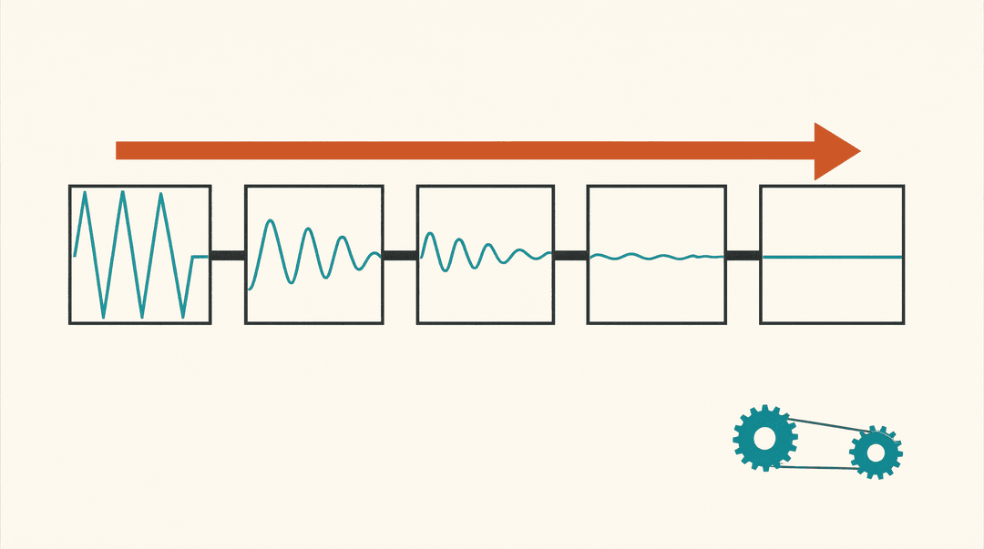
Consider one layer computing y = Wx, where x is a vector of d inputs and W is a matrix of weights. If the inputs have variance 1 and the weights are drawn with variance 1, the output variance scales with d. A layer with 512 inputs multiplies the signal variance by roughly 512. Stack ten such layers and the numbers grow by hundreds of billions. Run the same arithmetic in reverse and, with weights smaller than 1/d variance, the signal decays layer by layer until it is numerically zero.
The same chain rule that lets gradients flow backward also multiplies (or divides) them once per layer. Early networks therefore converged poorly in a direction-specific way: in deep sigmoid networks, gradients reaching the bottom layers were effectively zero, so early layers barely learned. This was formalized as the vanishing gradient problem in Hochreiter's 1991 work and the 1997 LSTM paper that was written to fix it for recurrent nets. The mirror image, exploding gradients, was analyzed by Pascanu, Mikolov and Bengio in 2013, who showed gradient norms in recurrent networks can grow exponentially and introduced gradient clipping as the standard patch.
Before 2010, the practical recipe was folklore: draw weights from a small uniform range, something like ±0.5, and hope. Small helped. It was not enough.
Xavier: pick the size from the layer's shape
In 2010, Glorot and Bengio published "Understanding the difficulty of training deep feedforward neural networks" (AISTATS), the paper that turned initialization into math. They derived the scale of the variance, not just its smallness.
Two conditions have to hold. To preserve signal variance going forward through a layer with n_in inputs, weights need variance 1/n_in. To preserve gradient variance going backward through a layer feeding n_out outputs, weights need variance 1/n_out. Both cannot hold at once unless the layer is square, so they averaged the two: variance 2/(n_in + n_out). For a uniform distribution that becomes the range ±sqrt(6/(n_in + n_out)), the formula that ships as "Xavier initialization," named after Glorot's first name.
Their experiments matched the theory: with tanh activations, their normalized initialization kept activations out of the saturating tails and kept gradient histograms roughly equal across layers, while the old small-random scheme let gradients shrink layer by layer. It also confirmed that the problem is not fully solved by initialization alone: very deep sigmoid nets still trained poorly, a finding that pushed the field toward better activations, better optimizers and, eventually, normalization layers.
He: ReLU throws away half the signal
By 2015 the state of the art ran on ReLU units, and Xavier's derivation quietly assumed activations that pass the whole input through. A ReLU zeroes out roughly half its inputs. The signal that does survive carries about half the variance Xavier budgets for it.
Kaiming He, Xiangyu Zhang, Jian Sun and colleagues derived the correction in "Delving Deep into Rectifiers" (ICCV 2015): double the variance, giving 2/n_in for a layer with n_in inputs. The paper states the practical difference bluntly: with their initialization, plain 30-layer rectifier networks could be trained from scratch, while the same deep plain networks "cannot" converge under Xavier. That capability was the precondition for He et al.'s ResNet, published months later, and the ImageNet results built on it briefly surpassed claimed human-level error on the benchmark. "Kaiming initialization," variance 2/fan_in with normal or uniform draws, is the default recommendation in PyTorch's own initialization documentation.
The lesson generalizes beyond ReLU: the correct variance is a property of the activation function sitting on top of the weight. Modern recipes plug in whatever activation the model actually uses, which is why GELU- and SwiGLU-era transformer papers still quote He-style constants.
The geometric school: orthogonal starts
A separate line of work argued that the distribution's shape matters more than its width. Saxe, McClelland and Ganguli analyzed deep linear networks in 2013 and found that learning speed is governed by the spectrum of singular values of the network's input-output Jacobian. Independent Gaussian draws smear that spectrum toward zero as depth grows; drawing each weight matrix from an orthogonal group (scaled appropriately) keeps singular values near 1 at all depths, giving "depth independent learning times," a property they named dynamical isometry. Orthogonal initialization and related unit-variance schemes like LSUV from Mishkin and Matas (ICLR 2016) tune the first batch of activations layer by layer instead of trusting a formula.
For production systems this school never displaced Xavier/He, but it explains a persistent observation: two initializations with the same per-weight variance can train at very different speeds, because what propagates through depth is not weights one at a time but products of whole matrices.
What actually ships: the GPT-2 compromise
Transformer language models are mostly LayerNorm-ed residual stacks, and LayerNorm rescales activations at every layer, which appears to make initialization a non-issue. The residual stream says otherwise. A residual block adds a function of the stream back onto the stream, so the variance of the stream grows monotonically with depth. By layer 60 you are summing 60 noisy contributions on top of the original embedding.
OpenAI's GPT-2 paper (Radford et al., 2019) handled this with an initialization-only fix: "We scale the weights of residual layers at initialization by a factor of 1/√N where N is the number of residual layers." Each branch writes a small correction into the stream instead of fighting it. The extra LayerNorm after the final block addresses the same accumulation from the other end.
That one sentence became the standard. Karpathy's nanoGPT, the reference implementation most hobbyists and many teams copy, initializes every linear layer with a normal distribution of std 0.02, then re-initializes every residual projection with std 0.02/sqrt(2 × n_layer) "per GPT-2 paper." A 12-layer model therefore starts with residual projections roughly five times smaller than its other linear layers.
Even the attention operation carries initialization DNA. The Vaswani et al. original Transformer paper divides query-key dot products by sqrt(d_k) precisely for the Glorot-Bengio reason: a d-dimensional dot product of unit-variance vectors has variance d, and unscaled logits push softmax into regions where gradients vanish. The 1/sqrt(d) in every attention head since is fan-in normalization wearing a different hat.
Why nobody fine-tunes this number by hand anymore
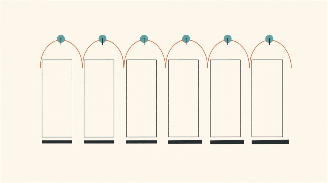
Three tools absorbed most of the pain that Xavier and He addressed. Batch normalization (Ioffe and Szegedy, 2015) re-standardizes activations every layer, which as the paper itself notes makes the network much less sensitive to initialization; vision CNNs largely stopped worrying. Residual connections gave gradients a highway that does not multiplicatively decay. Warmup schedules in Adam-era optimizers let early layers settle before full-strength updates.
What none of them fix is the first forward pass. At step zero, before any optimizer trick applies, the only thing standing between a deep model and a dead gradient is the scale of the numbers it was seeded with. That is also why initialization survives in every model card and training repo: it is cheap, it is deterministic once seeded, and getting it wrong is still the most common reason a from-scratch training run "just doesn't work." Allen-Zhu and Li's 2021 knowledge gap theory goes further, arguing that what a deep network can learn at all depends on functions reachable from its initialization, with some targets provably requiring exponential time from standard random starts.
The short version
A network starts as random numbers because symmetry must be broken. The numbers have to be the right size because layer chains multiply or divide signal and gradient once per layer, and the right size is computable from fan-in, fan-out and the activation function: Xavier's 2/(n_in+n_out), He's 2/n_in for ReLU, GPT-2's 1/√N for residual branches. Every large model you have used was seeded by some variation of these three formulas.
Sources
- Glorot & Bengio, "Understanding the difficulty of training deep feedforward neural networks," AISTATS 2010. https://proceedings.mlr.press/v9/glorot10a/glorot10a.pdf
- He, Zhang, Ren & Sun, "Delving Deep into Rectifiers: Surpassing Human-Level Performance on ImageNet Classification," ICCV 2015. https://arxiv.org/abs/1502.01852
- He, Zhang, Ren & Sun, "Deep Residual Learning for Image Recognition," CVPR 2016. https://arxiv.org/abs/1512.03385
- Saxe, McClelland & Ganguli, "Exact solutions to the nonlinear dynamics of learning in deep linear neural networks," 2013. https://arxiv.org/abs/1312.6120
- Mishkin & Matas, "All you need is a good init," ICLR 2016. https://arxiv.org/abs/1511.06422
- Pascanu, Mikolov & Bengio, "On the difficulty of training recurrent neural networks," ICML 2013. https://arxiv.org/abs/1204.2206
- Hochreiter & Schmidhuber, "Long Short-Term Memory," Neural Computation 1997. https://direct.mit.edu/neco/article/9/8/1735/6170/Long-Short-Term-Memory
- Radford et al., "Language Models are Unsupervised Multitask Learners," OpenAI 2019. https://cdn.openai.com/better-language-models/language_models_are_unsupervised_multitask_learners.pdf
- Vaswani et al., "Attention Is All You Need," NeurIPS 2017. https://arxiv.org/abs/1706.03762
- Ioffe & Szegedy, "Batch Normalization: Accelerating Deep Network Training by Reducing Internal Covariate Shift," ICML 2015. https://arxiv.org/abs/1502.03167
- Allen-Zhu & Li, "Physics of Language Models: Part 2.1, Knowledge and Reasoning," 2021. https://arxiv.org/abs/2104.10169
- Stanford CS231n notes, "Neural Networks: Training." https://cs231n.github.io/neural-networks-2/
- PyTorch docs, torch.nn.init. https://pytorch.org/docs/stable/nn.init.html
- Karpathy, nanoGPT model.py (GPT-2 style scaled residual init). https://github.com/karpathy/nanoGPT/blob/master/model.py
