
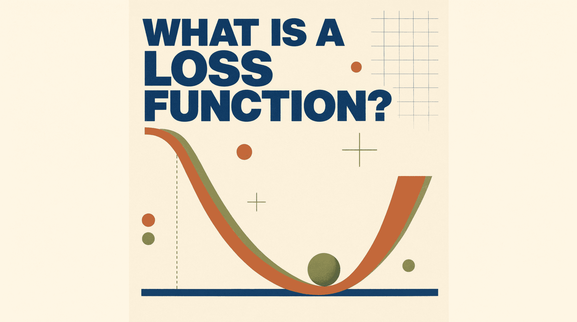
Every neural network, from a digit classifier on a laptop to a trillion-parameter language model, spends its training doing one thing: trying to make a single number smaller. That number is the loss, and the rule that turns the model's behavior into that number is the loss function. It is the most boring-sounding concept in deep learning and the one that quietly decides what a model becomes.
A loss function is a grading rule. The model produces outputs. The loss function compares those outputs against what the training data says should have happened and returns one real number, with lower always meaning better. Training, in the form of gradient descent, then nudges the model's weights in the direction that shrinks that number. The loss function is therefore the interface between a goal, which is fuzzy, and an optimizer, which only understands arithmetic. Whatever you want a model to learn, you have to be able to write down as a number. Misspecify the number and you get exactly what you asked for, which is rarely what you wanted.
The oldest loss is more than 200 years old
The default loss for regression problems, mean squared error, predates electricity. The method of least squares was first published by the French mathematician Adrien-Marie Legendre in 1805, in an appendix on computing comet orbits. Carl Friedrich Gauss had been using it since 1795 but did not publish until 1809, kicking off one of the most famous priority disputes in mathematics. Gauss made the method famous by predicting the orbit of the dwarf planet Ceres from a handful of observations; when it was rediscovered in December 1801, his numbers were by far the closest (Least squares, The Discovery of Statistical Regression).
The choice to square errors rather than take absolute values was not mystical. Squaring punishes big mistakes more than small ones, rewards the average rather than the median, and, crucially for the machine-learning era, produces a smooth curve that calculus can work with. When squaring punishes too hard, an extreme error dominates the entire fit. The standard fix is itself a designed loss function: in 1964 Peter Huber proposed a hybrid that is quadratic for small errors and only linear for large ones, trading accuracy on clean data for robustness against outliers (Huber, Annals of Mathematical Statistics, 1964, Robust regression). That compromise survives inside modern reinforcement learning: the PPO algorithm clips its value-function loss in a Huber-like way to keep rare, large errors from wrecking training (Schulman et al., 2017).
The number that punishes arrogance
Large language models use a different family of loss, rooted in information theory. Claude Shannon's 1948 paper defined entropy as the cost, in bits, of encoding outcomes from a distribution (Shannon, Bell System Technical Journal, 1948). The cross-entropy between the true next token and the model's predicted probability distribution turns out to reduce, in the one-hot case, to a remarkably simple expression: the loss at each position is just minus the logarithm of the probability the model assigned to the token that actually came next (Raschka, How does next-token prediction train a large language model?).
The log makes the grading rule severe in a useful way. If the model gives the correct token 99% probability, the loss is about 0.01. At 50%, the loss is 0.69. At 1%, it is 4.6. At 0.1%, it is 6.9. Honest uncertainty costs a little; confident wrongness costs a lot. This is why cross-entropy is also maximum likelihood: minimizing it across a corpus is identical to making the observed text as probable as possible, and it is equivalent to minimizing the Kullback-Leibler divergence between the model and the data (MLQ.ai, Pretraining: cross-entropy, perplexity, 6ND).
Two practical consequences follow. First, perplexity, the number researchers quote when comparing models on long-document tasks, is just the exponential of cross-entropy loss: an effective number of equally-likely choices per step. Second, you can predict what loss a brand-new model should print at step zero: the log of the vocabulary size, because a clueless model spreads probability uniformly. For GPT-2's 50,257-token vocabulary that is 10.8; for Llama 3's 128,256 tokens, 11.8. If a training run starts elsewhere, something in the setup is wrong before the first real update has even happened.

What loss curves are actually telling you
A pretraining run is a single loss number scrolling down on a dashboard, billions of dollars of compute measured as a slowly shrinking decimal. That number carries real information. The Kaplan scaling laws (2020) and the Chinchilla follow-up (2022) found that loss falls as a clean power law in parameters, data, and compute, which is why labs can spend months predicting what a bigger run will achieve before running it. Because training itself is just loss minimization, the whole economics of frontier model sizing hangs off that decimal.
But the number needs careful reading. Loss values from two models using different tokenizers are not directly comparable, because cross-entropy in nats-per-token depends on where each vocabulary cuts words; bits-per-byte normalizes that away (see our explainer on perplexity and bits-per-byte). And train loss alone hides the classic failure: a model can memorize its training data while getting no better on new text. That is why the diagnostic that matters is held-out loss, and why train loss falling while validation loss rises is the textbook signature of overfitting.
Different jobs need different rulers
The loss function is task-specific, and labs treat it as a design surface:
- Text generation uses cross-entropy on the next token, computed at every position of every training sequence in one pass (Raschka).
- Image generation by diffusion mostly uses plain mean-squared error between the noise a model predicts and the noise actually added to a training image. Notably, the DDPM paper found this simplified MSE worked better in practice than the principled variational bound it was derived from (Ho, Jain and Abbeel, 2020).
- RLHF skips labeled targets entirely. InstructGPT-style training optimizes a score from a learned reward model instead of a fixed loss on ground truth (Ouyang et al., 2022).
- Direct Preference Optimization converts preference pairs into an explicit loss function so alignment can be trained without a reward model in the loop (Rafailov et al., 2023).
The limits of the concept are the same as its power. A loss function only grades what it can see. Cross-entropy rewards text that is statistically like the corpus, not text that is true, which is one structural reason models hallucinate. Any proxy metric optimized hard enough can drift from the goal it stands in for; reward-model overoptimization, where a model games the reward instead of the intent, is the alignment-era version of that problem (Gao et al., 2023). Choosing the loss is choosing what the model will relentlessly, dumbly, and scalably pursue. Every capability in a modern AI system is downstream of somebody deciding what "less wrong" meant, writing it as a number, and getting out of gradient descent's way.
Sources
- Least squares, Wikipedia
- The Discovery of Statistical Regression, Priceonomics
- Huber, Robust Estimation of a Location Parameter, 1964
- Robust regression, Wikipedia
- Schulman et al., Proximal Policy Optimization Algorithms, 2017
- Shannon, A Mathematical Theory of Communication, 1948
- Raschka, How does next-token prediction train a large language model?
- MLQ.ai, Pretraining: Cross-Entropy, Perplexity, 6ND
- Kaplan et al., Scaling Laws for Neural Language Models, 2020
- Hoffmann et al., Training Compute-Optimal Large Language Models, 2022
- Ho, Jain and Abbeel, Denoising Diffusion Probabilistic Models, 2020
- Ouyang et al., Training language models to follow instructions with human feedback, 2022
- Rafailov et al., Direct Preference Optimization, 2023
- Gao et al., Scaling Laws for Reward Model Overoptimization, 2023
