
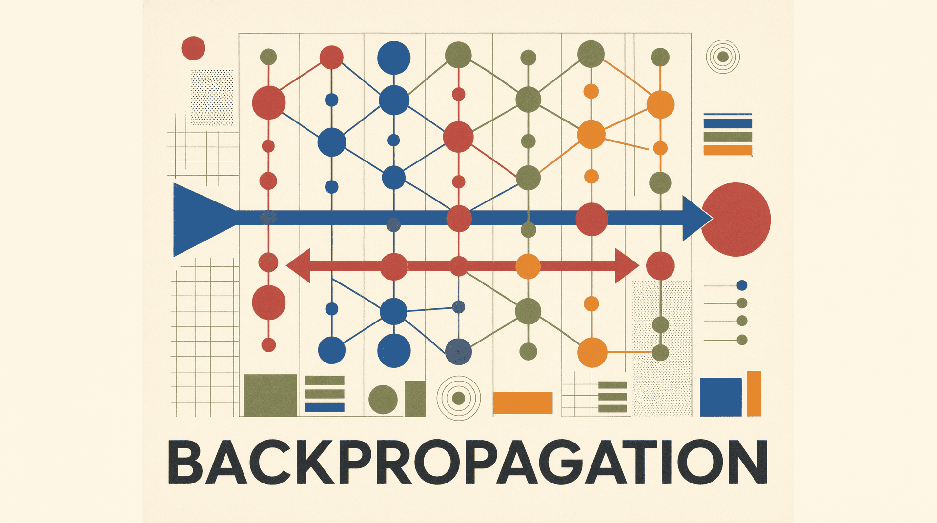
Every model release note mentions training tokens, training compute, or a post-training pipeline. Almost none explain the mechanism that does the actual learning. It is backpropagation: an algorithm from 1986, with precursors going back to the early 1960s, that remains the way essentially every neural network you have used got its weights. In October 2024 the Royal Swedish Academy awarded the Nobel Prize in Physics to John Hopfield and Geoffrey Hinton "for foundational discoveries and inventions that enable machine learning with artificial neural networks," and Hinton's citation rests partly on this algorithm.
The problem it solves
A neural network is a stack of layers, each layer a matrix of weights followed by a nonlinearity. Training means changing millions of those numbers so the network's output gets closer to the target. The difficulty is that only the final output is observable. If a language model produces a wrong prediction, the error is visible at the last layer, but the mistake was distributed across dozens of hidden layers in between. Which of the millions of weights is responsible, and by how much?
This is the credit assignment problem. Single-layer perceptrons had a direct learning rule; multilayer networks did not. Minsky and Papert's 1969 book Perceptrons highlighted the limits of single-layer machines, and the general problem of training layers in the middle stayed open through the 1970s. Backpropagation closed it: it computes, for every weight in every layer, exactly how much that weight contributed to the final error.
How it works
The procedure has three moves, repeated until the numbers stop improving.
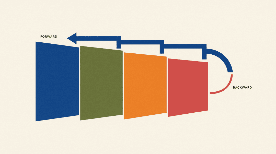
- Forward pass. The input runs through the layers and the network produces a prediction. The intermediate values computed along the way are kept, because the second move needs them.
- Backward pass. A loss function measures the gap between prediction and target. The algorithm then walks the computation in reverse, from the output back to the input, applying the chain rule of calculus one layer at a time. Each layer takes the error signal arriving from above, multiplies it by that layer's local derivatives, and passes a modified signal down to the previous layer. The output of this sweep is a gradient for every weight and bias in the network.
- Update. Each weight moves a small step in the direction that reduces the error: new weight equals old weight minus the learning rate times its gradient. The chain rule guarantees this is the correct local direction; the learning rate controls how far to trust it.
The trick is that the chain rule factors cleanly. The derivative of the loss with respect to a weight in layer three can be written as a product of terms, each of which was already computed while visiting layer four, five, and so on. Doing the bookkeeping once, right to left, yields gradients for all weights in a single sweep. The 1986 Nature paper by David Rumelhart, Geoffrey Hinton, and Ronald Williams framed it precisely this way: hidden units have no direct targets, so their error signals are computed indirectly from the units above them, and the weights are then adjusted by gradient descent.
A short history lesson
The 1986 paper is usually dated as the birth of backpropagation, and it is the version that convinced the field. It was not the first version. The mathematical lineage runs through control theory and automatic differentiation: Henry Kelley's 1960 method for two-point boundary value problems, Seppo Linnainmaa's 1970 master's thesis describing reverse-mode accumulation of derivatives, and Paul Werbos's 1974 Harvard PhD dissertation, which laid out the application to neural networks explicitly. Werbos's thesis sat largely unread for a decade. Rumelhart, Hinton, and Williams published a four-page letter in Nature, with experiments on training internal representations, and the idea took hold.
The first serious engineering applications followed quickly. In 1989 Yann LeCun, then at AT&T Bell Labs, published "Backpropagation Applied to Handwritten Zip Code Recognition": a network of about 1,250 units, roughly 65,000 connections, and fewer than 10,000 parameters, trained on some 7,300 handwritten ZIP code images from US Postal Service mail. It reached a 1% error rate, with about a 9% reject rate, on digits provided by the USPS. Karpathy's reproduction notes call it, to his knowledge, the earliest real-world application of a network trained with backpropagation. By the mid-2000s Hinton's layer-wise pretraining methods made deeper stacks trainable, and by 2012 the algorithm was training the networks that won ImageNet and started the modern deep learning era.

Backpropagation and large language models
Nothing about the algorithm changed when networks got bigger; only the scale did. Training a language model means running text through a transformer, computing the loss over the next-token predictions, sweeping gradients backward through every attention head and feed-forward matrix, and stepping the weights.
Two distinctions matter for reading model releases accurately.
First, backpropagation is not the whole training loop. It computes gradients; an optimizer such as SGD or Adam decides what to do with them, adding momentum, adaptive scaling, and weight decay. When a paper reports that training diverged at a learning-rate warmup, the gradients from backprop were fine; the update rule overshot.
Second, gradients require memory. The backward pass needs the intermediate values saved during the forward pass, which is why training consumes far more memory than inference and why techniques like activation checkpointing exist. Frameworks make this plumbing invisible on purpose: PyTorch's autograd engine records operations into a graph during the forward pass and differentiates it automatically on the backward pass, which is why researchers can change architectures freely without writing derivative code by hand.
The same algorithm sits under everything the site has explained recently. Fine-tuning is backprop on a smaller dataset. RLHF is backprop through a reward signal instead of a labeled target. Distillation is backprop against a teacher's outputs rather than a human's. The post-training methods differ; the learning mechanism does not.
Can anything replace it?
Backpropagation has known drawbacks. It is almost certainly not what brains do: computing exact error signals requires sending precise weight information backward through the network, something no one has demonstrated in biology. The 1986 paper itself conceded that "the learning procedure, in its current form, is not a plausible model of learning in brains." It also serializes training: each layer must wait for the gradient signal from the layers above it, and the saved activations cost memory.
Researchers have chased alternatives for a decade: feedback alignment, which substitutes random fixed backward weights; target propagation, which propagates activation targets instead of gradients; LeCun's Forward-Forward algorithm; and newer schemes such as NoProp, which trains each block with local denoising targets using neither a full forward nor a full backward pass. A 2020 NeurIPS analysis of target propagation put the state of the field plainly: these algorithms have not yet reached the performance of backpropagation. On small benchmarks like MNIST and CIFAR some alternatives now match it. On trillions of tokens, nothing has.
So the algorithm that made modern AI possible remains, four decades on, a slightly boring piece of calculus bookkeeping that nobody has beaten.
Sources
- Rumelhart, Hinton & Williams, "Learning representations by back-propagating errors," Nature, 1986: https://www.nature.com/articles/323533a0 (PDF mirror: https://gwern.net/doc/ai/nn/1986-rumelhart-2.pdf)
- Paul Werbos, "Beyond Regression" (1974 thesis history), Werbos.com: https://www.werbos.com/AD2004.pdf
- Harry Law, "Backpropagation is older than you think": https://www.learningfromexamples.com/p/backpropagation-is-older-than-you
- Wikipedia, "Backpropagation": https://en.wikipedia.org/wiki/Backpropagation
- LeCun et al., "Backpropagation Applied to Handwritten Zip Code Recognition," 1989: https://galileo-unbound.blog/wp-content/uploads/2025/02/lecun.neco_.1989.1.4.541.pdf
- Karpathy, lecun1989-repro notes: https://github.com/karpathy/lecun1989-repro
- Nobel Prize in Physics 2024: https://www.nobelprize.org/prizes/physics/2024/summary/
- PyTorch autograd documentation: https://docs.pytorch.org/docs/stable/notes/autograd.html
- Liu et al., "A Theoretical Framework for Target Propagation," NeurIPS 2020: https://proceedings.neurips.cc/paper/2020/file/e7a425c6ece20cbc9056f98699b53c6f-Paper.pdf
- "NoProp: Training Neural Networks without Back-propagation or Forward-propagation," arXiv 2025: https://arxiv.org/abs/2503.24322
