Test-Time Training (TTT): Mathematical Foundations, Expressive Hidden States, and Linear Complexity in Sequence Models

Sequence modeling has long been characterized by a sharp trade-off between computational efficiency and expressive memory. Transformers provide high expressive capacity by retaining all historical tokens in an uncompressed Key-Value (KV) cache. This structure enables them to scale to long contexts and continuously reduce perplexity as more tokens are conditioned on. However, this expressive power comes at the cost of quadratic computational complexity during prefill and linearly growing memory footprint during autoregressive decoding.

In contrast, Recurrent Neural Networks (RNNs) and State Space Models (SSMs), such as RWKV and Mamba, operate with linear computational complexity and constant inference memory. They achieve this by compressing history into a fixed-size hidden state. Yet, empirical evaluations demonstrate that fixed-size linear states struggle with long-range context utilization. As observed in scaling evaluations, architectures like Mamba often see perplexity gains plateau beyond 16,000 tokens on long-context benchmarks such as Books.

Test-Time Training (TTT), introduced by researchers from UC Berkeley, Stanford, UCSD, and Meta (Sun et al., 2024), resolves this trade-off. Instead of treating the hidden state as a passive vector or static matrix, TTT defines the hidden state as the weights of an internal machine learning model. Updating the hidden state during inference becomes an explicit step of self-supervised gradient descent. This architecture achieves linear computational complexity, constant per-step generation memory, and expressive capacity that matches Transformers across long sequences.

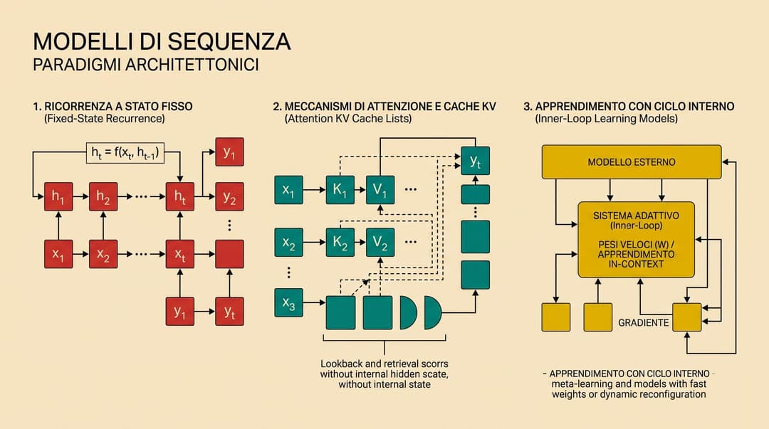
The Hidden State as a Machine Learning Model

All autoregressive sequence modeling layers map an input sequence x_1, ..., x_T to an output sequence z_1, ..., z_T by maintaining some representation of context. The design of that context representation dictates both computational efficiency and expressive limits:

• Standard RNNs maintain a fixed-size vector s_t in R^d, updated via s_t = sigma(W_ss s_{t-1} + W_sx x_t). The update and output rules require O(1) compute per token, but the vector bottleneck restricts long-term associative memory.
• Self-Attention maintains an unbounded list of keys and values, s_t = [(k_1, v_1), ..., (k_t, v_t)]. The output rule z_t = V_t softmax(K_t^T q_t) requires O(t) compute per token, retaining all historic context without lossy compression.
• TTT layers set the hidden state s_t equal to W_t, the parameters of an inner-loop prediction model f. The update rule is a step of gradient descent on a self-supervised objective, and the output rule evaluates f on the current token representation.

The intuition behind TTT originates from parametric learning: neural network pre-training is itself a lossy compression heuristic. When an LLM is trained on internet data, billions of tokens are compressed into weight matrices that capture complex relationships and structure. TTT applies this compression mechanism at the sequence level. By treating an input sequence as an unlabeled dataset and the layer's hidden state as a learner, the model uses gradient descent to store context into weights.

The basic formulation of a TTT layer proceeds as follows:

• Output rule: z_t = f(x_t; W_t)
• Update rule: W_t = W_{t-1} - eta nabla ell(W_{t-1}; x_t)

Here, W_0 is the base state (typically initialized to zero or a learned prior), eta is the inner-loop learning rate, and ell is an internal self-supervised loss function. Tokens that generate larger gradients induce greater weight changes, prioritizing information that the current weights fail to predict.

Nested Optimization: Inner and Outer Loops

A network equipped with TTT layers operates via two nested learning problems: an inner loop that runs per sequence, and an outer loop that trains the entire architecture.

• Inner loop: Operates during both training and inference. For each token x_t in a sequence, the inner loop computes the gradient of a self-supervised task with respect to the hidden state weights W, updating W_t dynamically.
• Outer loop: Operates during standard model pre-training. It updates the global model parameters theta_{rest} via cross-entropy loss on next-token prediction across the broader training corpus.

Multi-View Self-Supervised Reconstruction

To drive the inner loop without external labels, TTT formulates a self-supervised reconstruction task. A naive autoencoding loss ||f(x_t; W) - x_t||^2 is suboptimal because raw input tokens contain noise that should not be retained.

TTT addresses this by parameterizing the self-supervised task with learned projections, termed multi-view reconstruction:

• Training view: x_tilde_t = theta_K x_t (specifying the corrupted input to f)
• Label view: y_t = theta_V x_t (specifying the target feature representation to reconstruct)
• Test view: q_t = theta_Q x_t (specifying the query representation used to produce the layer output)

The matrices theta_K, theta_V, and theta_Q are outer-loop parameters optimized end-to-end alongside the rest of the network. The inner-loop objective is:

ell(W; x_t) = || f(theta_K x_t; W) - theta_V x_t ||^2

The output rule evaluates the inner model on the test view:

z_t = f(theta_Q x_t; W_t)

This formulation establishes an explicit structural analogy with Self-Attention: theta_K, theta_V, and theta_Q serve the roles of Key, Value, and Query projection matrices. However, instead of computing pairwise dot-product attention scores across an expanding cache, theta_K and theta_V parameterize a self-supervised regression problem solved by gradient descent.

Model Instantiations: TTT-Linear and TTT-MLP

The inner model f determines the representational capacity of the hidden state. The authors introduce two primary instantiations:

TTT-Linear

In TTT-Linear, the model f is a single linear projection: f(x; W) = W x, where W in R^{d_out x d_in}. The reconstruction loss simplifies to:

ell(W; x_t) = || W theta_K x_t - theta_V x_t ||^2

The gradient with respect to W is:

nabla ell(W; x_t) = 2 (W theta_K x_t - theta_V x_t) (theta_K x_t)^T

TTT-MLP

In TTT-MLP, f is a two-layer multi-layer perceptron with hidden dimension 4d, GELU activations, layer normalization, and a residual connection:

f(x; W) = x + W_2 GELU(LN(W_1 x))

By employing a non-linear network inside the hidden state, TTT-MLP expands the expressive capacity beyond standard bilinear associative memories. It enables the hidden state to model multi-stage functional dependencies within the context window.

Mathematical Equivalence to Linear Attention

TTT provides a theoretical bridge connecting gradient descent to existing recurrence mechanisms.

Theorem: Consider a TTT-Linear layer where f(x) = W x, initialized with W_0 = 0. If the update rule uses batch gradient descent with learning rate eta = 1/2 over all prior tokens, the output sequence z_1, ..., z_T is mathematically identical to standard Linear Attention.

Proof summary: Under batch gradient descent from W_0 = 0, the accumulated gradient over preceding tokens evaluates to:

nabla ell(W_0; x_s) = -2 (theta_V x_s) (theta_K x_s)^T = -2 v_s k_s^T

Accumulating these updates yields:

W_t = W_0 - eta sum_{s=1}^t nabla ell(W_0; x_s) = sum_{s=1}^t v_s k_s^T

Evaluating the output rule on query q_t = theta_Q x_t yields:

z_t = W_t q_t = (sum_{s=1}^t v_s k_s^T) q_t = sum_{s=1}^t v_s (k_s^T q_t)

This matches the exact definition of Linear Attention without softmax (Katharapu et al., 2020).

However, Linear Attention represents a restricted degenerate case: it corresponds to taking only a single batch gradient step from zero. In practice, TTT-Linear employs multi-step online or mini-batch gradient descent. Each step updates weights relative to the previous step's parameters W_{t-1}, allowing the state to move dynamically through parameter space rather than staying fixed to a one-step projection.

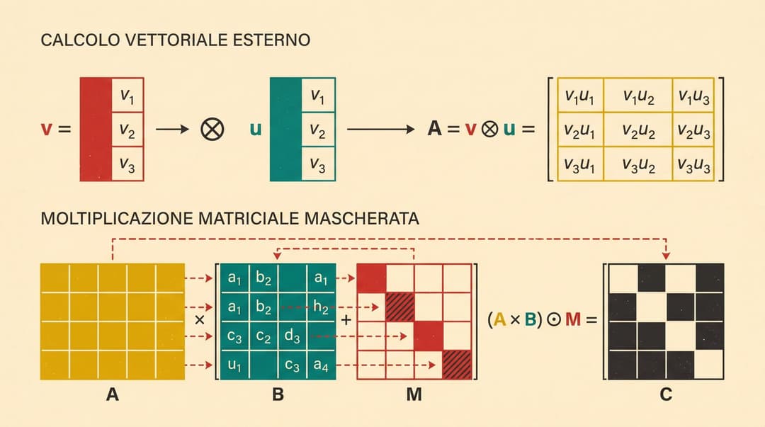
Hardware Efficiency: Mini-Batch TTT and the Dual Form

A naive implementation of online gradient descent is computationally inefficient on modern accelerators. Sequential outer products G_t = nabla ell(W_{t-1}; x_t) cannot saturate GPU TensorCores, which require dense matrix multiplications (GEMMs). Furthermore, materializing intermediate weight matrices W_t in R^{d x d} for every token incurs excessive memory bandwidth overhead.

TTT addresses these hardware bottlenecks through two mathematical innovations:

1. Mini-Batch Gradient Descent

Instead of updating W token-by-token (online GD) or taking all gradients from W_0 (batch GD), TTT partitions the sequence into mini-batches of size b (typically b = 16). Within each mini-batch, gradients are evaluated with respect to the weight checkpoint at the start of that batch, denoted W_{t'}:

G_t = nabla ell(W_{t'}; x_t)

This allows b gradient updates to be calculated concurrently in parallel across tokens, preserving multi-step optimization dynamics across the sequence while enabling intra-batch parallelism.

2. The Dual Form

To avoid explicitly instantiating the intermediate weight updates G_1, ..., G_b during sequence processing, TTT derives a dual representation using Gram matrix formulations.

Let X = [x_1, ..., x_b] represent the batched token inputs, with theta_K = theta_V = theta_Q = I for exposition. The weight tensor at the conclusion of a mini-batch of size b is:

W_b = W_0 - 2 eta (W_0 X - X) X^T

This operation computes W_b using two standard GEMM operations.

To compute the intermediate token outputs Z = [z_1, ..., z_b] without materializing intermediate W_t states, the inner products between tokens are computed via a masked Gram matrix:

Delta = mask(X^T X) (W_0 X - X)

Here, mask denotes a strictly lower-triangular causal mask where non-causal entries are set to zero. The output tokens are then computed directly:

Z = W_0 X - 2 eta Delta

While the theoretical FLOP count of the dual form includes an O(b^2 d) term for the token attention-like matrix, setting b = 16 keeps this overhead negligible. More importantly, it converts memory-bound outer products into hardware-aligned GEMMs. In JAX benchmarks on TPU and GPU clusters, the dual form accelerates training by more than 5x compared to the primal form, matching the execution speed of highly optimized Mamba kernels.

Empirical Findings and Scaling Characteristics

Sun et al. evaluated TTT-Linear and TTT-MLP against Transformer and Mamba architectures across parameter scales from 125M to 1.3B:

• Context length scaling: On long-context modeling benchmarks (such as Books at 32k context), Transformer and TTT variants continuously decrease validation perplexity across the entire sequence length. In contrast, Mamba's perplexity reduction plateaus after 16k tokens, unable to compress longer dependencies into a static recurrence state.
• Efficiency at scale: At 8,000 tokens, TTT-Linear matches the wall-clock training and inference speed of Mamba, while running faster than FlashAttention-2 Transformers.
• Expressive capacity: TTT-MLP demonstrates stronger long-context utilization than TTT-Linear, showing lower perplexity as sequence length expands. However, due to the non-linear transformations inside the inner loop, TTT-MLP requires higher memory I/O and custom kernel development to match TTT-Linear's wall-clock throughput.

Outlook and Architectural Significance

Test-Time Training establishes a new conceptual foundation for sequence modeling:

1. Unified framework: TTT demonstrates that recurrence, linear attention, and meta-learning can be expressed within a single mathematical formulation governed by gradient descent on self-supervised objectives.
2. Constant memory inference: By storing contextual history in weights rather than an expanding KV cache, TTT models execute autoregressive generation in O(1) memory per step, eliminating KV-cache memory exhaustion during long-context deployment.
3. Expressive compression: By substituting fixed linear recurrent updates with multi-layer neural network parameters, TTT circumvents the historical compression bottleneck that constrained earlier RNN architectures.

As context windows scale to millions of tokens, the boundary between in-context learning and weight optimization is blurring. TTT offers a principled, hardware-efficient path toward sequence architectures that scale linearly without sacrificing memory capacity.

Sources

• Learning to (Learn at Test Time): RNNs with Expressive Hidden States (Sun et al., 2024)
• Official PyTorch Implementation of TTT-LM
• Official JAX Implementation of TTT-LM
• Mamba: Linear-Time Sequence Modeling with Selective State Spaces (Gu & Dao, 2023)
• Transformers are RNNs: Fast Autoregressive Transformers with Linear Attention (Katharapu et al., 2020)
• Deep Learning with Test-Time Training: A Survey