
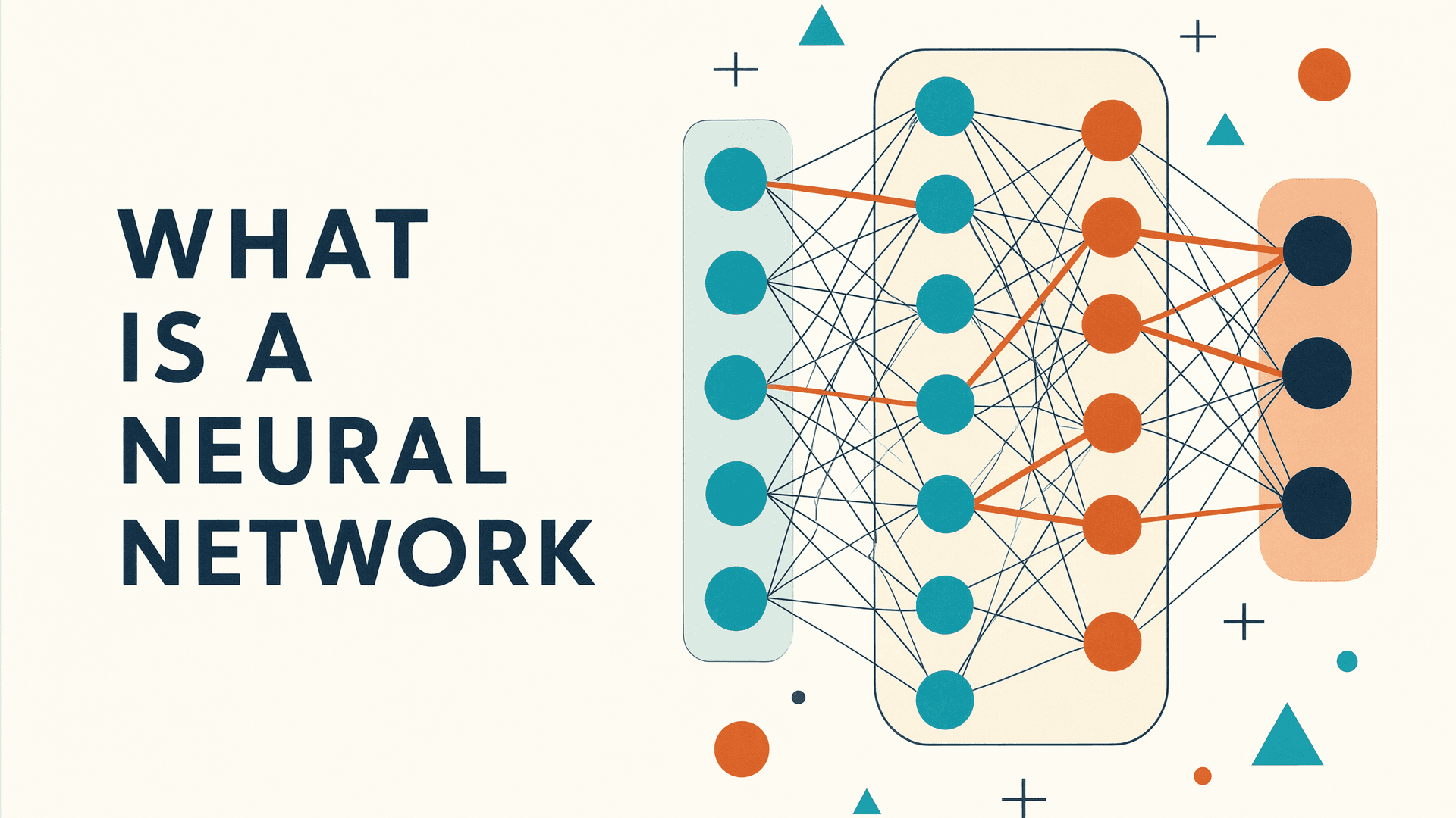
Every language model you have used is a neural network. The phrase sounds biological, but the thing itself is arithmetic: a stack of weighted sums, nonlinear bumps and more weighted sums, tuned until the output matches what was wanted. This explainer covers what a neural network is, where the idea came from, why it took 54 years to take over the field, and what the stack looks like inside a modern LLM.
The original unit: a weighted sum with a decision
In 1958, the psychologist Frank Rosenblatt demonstrated a learning machine he called the perceptron. The demonstration ran in simulation on an IBM 704, a 5-ton room-sized computer that sorted punch cards after roughly 50 tries, and the Office of Naval Research announced it at a press conference that July, describing it as "the first machine which is capable of having an original idea" (Cornell Chronicle). Rosenblatt's team later built a dedicated hardware version, the Mark I Perceptron, at the Cornell Aeronautical Laboratory in Buffalo and demonstrated it publicly in 1960, with motor-driven potentiometers standing in for adjustable weights (Wikipedia).
A perceptron does one thing. It takes inputs, multiplies each by a learned weight, adds them up, and compares the total to a threshold to produce a yes/no answer. If the answer is wrong, a simple rule nudges the weights toward the correct answer. Rosenblatt proved the procedure converges: if a set of weights that solves the problem exists, the learning rule finds it in a finite number of steps.
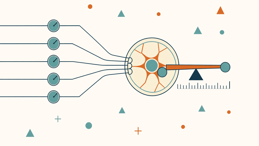
One perceptron can only draw a straight line (or, in high dimensions, a flat plane) between the categories it separates. That limitation is the entire plot of the next three decades.
Why one layer was not enough
In 1969, Marvin Minsky and Seymour Papert published Perceptrons, a rigorous analysis showing that single-layer machines cannot even solve simple problems like XOR, where the two categories are laid out diagonally. No amount of straight-line geometry separates them (MIT Press). The book is routinely cited as a cause of the first AI winter, the long pullback in funding for connectionist research that followed.
The fix was depth. Put multiple perceptrons in layers, feed the outputs of one layer into the next, and the network can fold space: the second layer draws lines through a world the first layer has already bent. Three results made this precise.
First, the learning problem. To train a deep network you need to know how each weight in each layer contributed to the final error. The answer, backpropagation, applies the chain rule from calculus to push error signals backward through the layers, adjusting every weight in proportion to its blame. The procedure that made the field use it was described in 1986 by David Rumelhart, Geoffrey Hinton and Ronald Williams in Nature (Rumelhart, Hinton & Williams, 1986).
Second, the capability problem. In 1989, Kurt Hornik, Maxwell Stinchcombe and Halbert White proved the universal approximation theorem: a feedforward network with even a single hidden layer can approximate any continuous function to any desired accuracy, given enough units (Hornik et al., 1989). The theorem says deep networks can represent almost anything. It says nothing about whether you can find the right weights, and it gives no useful bound on how many units "enough" means.
Third, the practical machinery. Over the 1990s and 2000s, Yann LeCun's group and others trained real networks on real tasks like handwritten digit recognition, but training stalled as layers stacked up. Fixes arrived piecemeal: better activation functions such as the rectified linear unit (ReLU), introduced to machine learning by Nair and Hinton in 2010 (ICML 2010), and regularizers like dropout (NeurIPS 2012 paper).
2012: the year the stack won
The turn came at the ImageNet competition in 2012. ImageNet's ILSVRC track offered roughly 1.2 million labeled images across 1,000 categories, enough data to train a deep network end to end. A team from the University of Toronto, Alex Krizhevsky, Ilya Sutskever and Geoffrey Hinton, entered an eight-layer convolutional network later known as AlexNet. Its top-5 error was 15.3 percent. The second-place entry managed 26.2 percent (Krizhevsky, Sutskever & Hinton, NeurIPS 2012). The gap was larger than several years of gradual progress by conventional methods, and it ended the debate.
The paper's own account of why it worked is unromantic. Three ingredients met at once: a large labeled dataset, GPUs as cheap parallel compute (the model was trained on two Nvidia GeForce GTX 580 cards over five to six days), and training tricks like ReLU and dropout that kept deep networks trainable. Neural networks did not suddenly become smarter. The conditions for actually fitting them became available.
Inside a language model
A modern LLM is the same stack, shaped for sequences of tokens. Input text is cut into tokens, each mapped to a vector of numbers, and the vectors pass through dozens of layers. Each layer is mostly two parts: a mechanism that mixes information across positions (attention, in transformers) and a feed-forward neural network applied to each position. The feed-forward part is a classic neural network: multiply by a weight matrix, bend with a nonlinearity, multiply again.
The scale is the difference from 2012. GPT-3, published in 2020, has 96 transformer layers and 175 billion parameters (Brown et al., 2020). Llama 3 405B, published in 2024, has 126 layers with 80 attention heads (Meta AI, 2024).
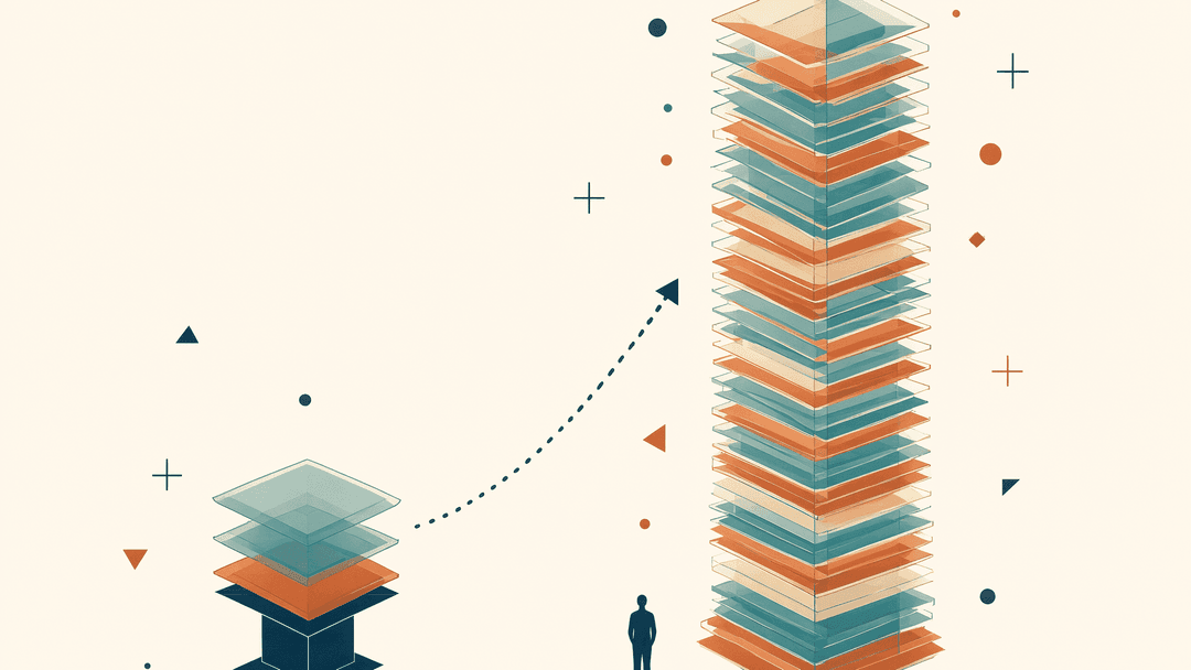
A "parameter" is one number in one of those weight matrices, and training is backpropagation at this scale: forward pass to compute the error on the next token, backward pass to assign blame across 400-odd billion numbers, then a small gradient-descent step on all of them at once. For those pieces separately, see What Are Model Parameters?, What Is Backpropagation? and What Is Gradient Descent?.
What a neural network is not
Two caveats worth keeping in view. The neurons in a neural network are named after the biological thing and nothing more; the model is not simulating cells, and the learning rule bears little resemblance to how synapses change. And the universal approximation theorem is a promise about representation, not about training: knowing that a network of a certain size could represent a function tells you nothing about whether gradient descent, a dataset and a budget of GPU-years will ever find it. Most of the engineering history of deep learning is about that gap.
The honest summary: a neural network is a function with millions of adjustable knobs, built so that calculus can tell you which knob to turn. That property, plus data and GPUs, is what turned a 1958 curiosity into the dominant technology of the last decade.
Sources
- Cornell Chronicle: Professor's perceptron paved the way for AI, 60 years too soon
- Wikipedia: Mark I Perceptron
- MIT Press: Perceptrons, Minsky & Papert, 1969
- Rumelhart, Hinton & Williams: Learning representations by back-propagating errors, Nature 323, 1986
- Hornik, Stinchcombe & White: Multilayer feedforward networks are universal approximators, Neural Networks 2, 1989
- Nair & Hinton: Rectified Linear Units improve Restricted Boltzmann Machines, ICML 2010
- Krizhevsky, Sutskever & Hinton: ImageNet Classification with Deep Convolutional Neural Networks, NeurIPS 2012
- Brown et al.: Language Models are Few-Shot Learners (GPT-3), 2020
- Meta AI: The Llama 3 Herd of Models, 2024
