

A training run does not end with one model. It ends with two: the weights the optimizer last touched, and a slower, smoothed copy that was quietly maintained beside it the whole time. In a lot of modern codebases, the second copy is the one that gets evaluated, published, and shipped. That copy is called the exponential moving average of the weights, or EMA, and it is one of the oldest tricks in optimization wearing one of the least-explained hats in deep learning.
The mechanism in one line
After every optimizer step, the shadow weights absorb a small fixed fraction of the live weights:
theta_EMA = beta * theta_EMA + (1 - beta) * theta_model
That is the entire algorithm. The decay factor beta sits between 0 and 1 and controls how much history the shadow model remembers. At beta = 0.9999, each update moves the average one ten-thousandth of the way toward the current weights, so the model you get reflects roughly the last 10,000 steps of training. Practical recipes cluster in that range. The Improved DDPM paper from OpenAI states plainly that most of its experiments used an EMA over model parameters with a rate of 0.9999, and the popular timm training library exposes exactly this update as an opt-in flag with the same style of decay.
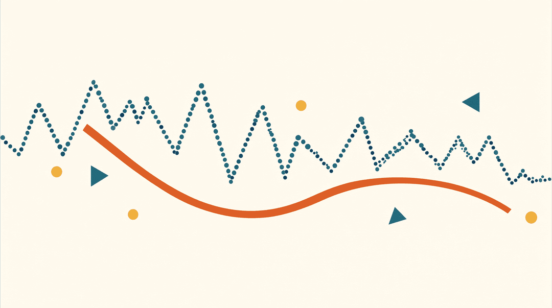
The intuition is statistical. Stochastic gradient descent does not glide to a minimum; it jitters around one, because each minibatch gradient is a noisy estimate of the true gradient. The final iterate is therefore one noisy sample drawn from the cloud of weights the optimizer explored near the end of training. An average of that cloud is a better estimate of its center than any single draw from it, and averaged weights tend to sit in flatter, more forgiving regions of the loss landscape.
Where the idea came from
Weight averaging predates deep learning by decades. Polyak and Juditsky showed in 1992 that averaging the last iterates of stochastic approximation cancels gradient noise and recovers the optimal convergence rate without shrinking the step size. In 2018, Izmailov and colleagues brought the idea into the transformer-era toolbox with Stochastic Weight Averaging (SWA), which uniform-averages checkpoints along an SGD trajectory and demonstrated that the averaged model finds visibly wider optima and generalizes better than the last iterate on CIFAR and ImageNet.
EMA is the online cousin of SWA. Instead of collecting discrete snapshots and averaging them at the end, it folds each new iterate into a running average every step, with exponentially decaying weight on the past. That makes EMA usable during training, not just after it, which is what turned it into infrastructure.
What the averaged model is actually good for
The most systematic evidence comes from a 2024 study by Morales-Brotons, Vogels and colleagues, which isolated EMA from the pipelines that usually hide it. Their findings, replicated across image classification benchmarks:
- EMA models generalize better than the last-iterate model, and they differ from it. This is not a rounding effect; the two solutions land in different places.
- EMA reduces the need for the end-of-training learning-rate decay. Because averaging cancels gradient noise itself, the EMA copy stays accurate at learning rates where plain SGD has stopped making progress. The authors propose it as a way to skip the final low-learning-rate phase of a run.
- The averaged model is measurably more robust to mislabeled data, better calibrated, and more consistent in its predictions. A high-learning-rate trajectory with noise memorizes wrong labels late in training; the average is slower to absorb that memorization.
- EMA performance peaks early and impressively, which the authors argue is a key reason EMA teachers work so well in student-teacher training.
That last point explains EMA's second life: as a target network. Mean Teacher (2017) first used an EMA of a model's own weights as a stable teacher for semi-supervised learning. BYOL (2020) built its entire self-supervised objective on a target network whose weights are an EMA of the online network, with no negative pairs at all. MoCo renamed the mechanism the "momentum encoder." DINO, the self-distillation recipe behind many vision foundation models, observed during training that the EMA teacher consistently outperforms the student it is derived from. On the generative side, the consistency models paper (2023) distills slow diffusion samplers into fast ones using an EMA target network, and separately applies EMA to the online weights themselves. StyleGAN2, the model that made photorealistic face generators credible, reports results using an exponential moving average of the generator weights, a practice it inherited from the earlier StyleGAN line.
The pattern across all of these: wherever you need a version of a model that changes slowly and predicts consistently while the real model is thrashing at a high learning rate, an EMA copy gives you one for free.
The costs and the fine print
Keeping a shadow model is not literally free. It is a second copy of every parameter, which for a frontier-scale network is a second copy of hundreds of gigabytes, plus a small per-step update cost. Teams that care about that memory either update the EMA every k steps (the 2024 study found sampling every few steps costs nothing in quality if you adjust the decay to compensate) or skip EMA entirely.
There is a well-documented trap with Batch Normalization. The BN running statistics of an EMA model go stale in a way the weights do not. Morales-Brotons and colleagues found that BN stats, not the weights, are the limiting factor on how slow you can set the decay: with a very large averaging window the EMA model diverges, until the BN statistics are recomputed over the training set, at which point the same window works and even improves results.
And EMA is not automatically the right averaging scheme for LLM pre-training. Sanyal, Kaddour and colleagues (2023) tested checkpoint averaging at language-model scale and found that at the high learning rates LLM training actually uses, averaging snapshots taken with considerable spacing between them outperformed both EMA and SWA baselines. Their recipe, built on the "latest weight averaging" idea, beat conventional training and its moving-average baselines on nanoGPT-2 models at 125M and 335M parameters. The lesson is that averaging works, but the window shape interacts with the optimizer, the batch size, and the learning-rate schedule.
Why it deserves a place in your vocabulary
Three concrete takeaways. First, when a training codebase ships an "eval checkpoint," "inference checkpoint," or "teacher," check whether it is an EMA copy; the numbers in the paper may describe a model that never existed at any single step of training. Second, if you fine-tune a model at an aggressive learning rate, keeping an EMA copy and early-stopping on it is one of the cheapest quality upgrades available, no architecture changes, no new data. Third, treat "the trained weights" as ambiguous. A training run is a trajectory, and any honest description of the endpoint should say which point on that trajectory, or which average over it, you decided to keep.
Sources
- Polyak and Juditsky, "Accelerating stochastic gradient descent methods by averaging of iterates" (1992), summarized with full history in Exponential Moving Average of Weights in Deep Learning: arXiv:2411.18704
- Morales-Brotons, Vogels et al., "Exponential Moving Average of Weights in Deep Learning: Dynamics and Benefits": arXiv:2411.18704
- Izmailov et al., "Averaging Weights Leads to Wider Optima and Better Generalization" (SWA): arXiv:1803.05407
- Sanyal et al., "Early Weight Averaging meets High Learning Rates for LLM Pre-training": arXiv:2306.03241
- Nichol and Dhariwal, "Improved Denoising Diffusion Probabilistic Models" (EMA rate 0.9999, Appendix): arXiv:2102.09672
- Grill et al., "Bootstrap Your Own Latent" (EMA target network): arXiv:2006.07733
- He et al., "Momentum Contrast" (MoCo momentum encoder): arXiv:1911.05722
- Caron et al., "Emerging Properties in Self-Supervised Vision Transformers" (DINO EMA teacher): arXiv:2104.14294
- Song et al., "Consistency Models" (EMA target for distillation): arXiv:2303.01469
- Karras et al., "Analyzing and Improving the Image Quality of StyleGAN" (EMA of generator weights): arXiv:1912.04958
- Tarvainen and Valpola, "Mean teachers are good role models": arXiv:1703.05175
timmModel EMA implementation guide: timm.fast.ai/training_modelEMA
