
Most of the current AI conversation is about language models. But when a system generates a photograph-grade image or a clip of video, an older architecture usually does part of the work: the variational autoencoder, VAE for short. It compresses pixels into a small, tidy mathematical space, and it expands them back out again. The generative model itself, whether it is a diffusion model or an autoregressive network, then operates on the compressed representation because raw pixels are too expensive to model directly.
This explainer covers what a VAE is, the specific 2013 trick that made it trainable, the failure modes it introduced, and where it sits in the AI stack today.
Start with the plain autoencoder
An autoencoder is a neural network with two halves. The encoder squeezes an input, say a 28-by-28 pixel digit, into a short code. The decoder tries to reconstruct the original image from that code alone. Training rewards accurate reconstruction, so the network is forced to keep the information that matters and discard the rest. No labels are required; the data supplies its own targets.
The architecture is old, and one result helped launch the modern deep learning era. In 2006, Geoffrey Hinton and Ruslan Salakhutdinov published Reducing the Dimensionality of Data with Neural Networks in Science. Their deep autoencoder learned to convert each 784-pixel MNIST image into six real numbers that allowed near-perfect reconstruction, while principal component analysis, the standard linear method, gave much worse reconstructions. The paper's contribution was an initialization scheme, training one layer at a time, that made gradient descent work on networks this deep.
Plain autoencoders have a limitation that matters for generation. The code is a point, not a region. If the encoder maps cats to one spot in code space and dogs to another, the halfway point between them is whatever the decoder happens to produce there, and nothing in training forces that in-between territory to be meaningful. Codes learned this way leave holes: points between them decode to mush.
The 2013 change: compress into a cloud, not a point
In December 2013, Diederik Kingma and Max Welling posted Auto-Encoding Variational Bayes (published at ICLR 2014). The paper asked how to do efficient inference and learning in models with continuous latent variables when the true posterior is intractable, which is the normal case for real data. Their answer was the variational autoencoder, and the construction has three moving parts.
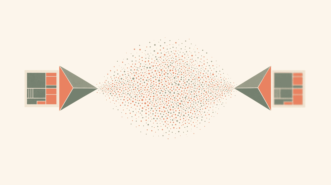
First, the encoder does not output a code. It outputs the parameters of a probability distribution over codes: typically a mean and a variance per latent dimension. Each image becomes a cloud of likely codes rather than a single point.
Second, a sample is drawn from that cloud and handed to the decoder, which reconstructs the input from the noisy code. Because the reconstruction must survive a random perturbation of its latent code, similar inputs are pushed to overlap rather than sit in isolated points. The latent space comes out smooth by design.
Third, the training objective has two terms, and together they form what is called the evidence lower bound, or ELBO. The reconstruction term rewards faithful decoding. The regularization term is a Kullback-Leibler divergence that pulls each input's cloud toward a fixed prior, conventionally a standard Gaussian. Carl Doersch's tutorial explains the mechanics in detail: the KL term keeps the clouds anchored near the prior, the reconstruction term keeps them distinguishable, and the tension between them is the whole model.
Sampling normally blocks gradient-based training, because a discrete draw from a distribution has no useful derivative with respect to the encoder's weights. The paper's key contribution was the workaround now called the reparameterization trick. Instead of sampling from the encoder's distribution directly, you take standard noise, draw it from a fixed Gaussian, and compute the code deterministically as mean plus standard deviation times noise. The randomness moves to a source the network does not touch, and gradients for the mean and the variance flow cleanly through the rest of the computation. That single reformulation is why VAEs train with ordinary stochastic gradient descent like any other network.
Doersch wrote in 2016 that in just three years VAEs had become one of the most popular approaches to unsupervised learning of complicated distributions, with results on digits, faces, scenes and video prediction. For a while, they were the default generative model.
Two ways it breaks
VAEs came with well-documented weaknesses, and understanding them explains why the field moved on.
The first is blurry output. A VAE decoder reconstructs an expectation over a noisy code, and the average of plausible images looks soft next to the sharp, mode-seeking samples a GAN produces. Lilian Weng's survey of the family walks through how the reconstruction term drives this behavior. The samples are diverse and the latent space is navigable, but pixel-level sharpness was never the VAE's strength.
The second is posterior collapse. The KL term is happy with a lazy solution: if the encoder outputs the prior for every input, the KL term goes to zero, and a powerful enough decoder can reconstruct the data on its own, ignoring the latent code entirely. The model then has a latent space that does nothing. The effect is most visible in text: researchers found that VAEs with autoregressive decoders routinely suffered posterior collapse, so the model degenerated into a plain language model, because a strong decoder makes the latent variable optional.
Two 2017 variants attacked these problems directly. DeepMind's beta-VAE put an adjustable weight on the KL term. With the pressure turned up past one, the model squeezed more of the data's independent structure, such as object pose and color, into separate latent dimensions, and it outperformed vanilla VAEs and InfoGAN on disentanglement benchmarks. The VQ-VAE, Neural Discrete Representation Learning from Van den Oord and colleagues at DeepMind, replaced the continuous Gaussian cloud with codes drawn from a learned book of discrete vectors, sidestepping posterior collapse when paired with strong autoregressive decoders. The VQ-VAE abstract claimed generation of high-quality images, video and speech, and unsupervised learning of phonemes from raw audio. That discrete-codebook lineage is the direct ancestor of the neural audio codecs modern speech models run on.
Where VAEs live in the current stack
The VAE never really retired; it moved under the things that did.
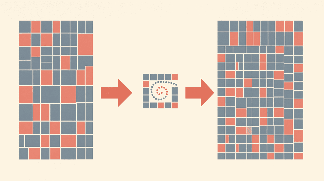
Latent diffusion models, the December 2021 paper by Rombach and colleagues, made the argument explicit. Diffusion models operating in pixel space needed hundreds of GPU days to train, so the authors ran the diffusion process in the latent space of a pretrained autoencoder instead, arguing that this hits a near-optimal point between complexity reduction and detail preservation. That paper is the architecture behind Stable Diffusion, released August 22, 2022, and the compressed-latent design became standard across image generation. Every Stable Diffusion style pipeline still encodes the prompt's future image through an autoencoder and decodes the diffusion result back into pixels.
Video went the same way. Wan, Alibaba's open video generation suite from 2025, lists a novel VAE among its four key features and credits the compression work in part for a 1.3B model that runs in 8.19 GB of VRAM. A minute of raw 1080p video is enormous; a video VAE shrinks it by orders of magnitude so a diffusion transformer can afford to model it.
For readers focused on language models, the practical takeaways are smaller but real. VAEs are not in the transformer loop, but their ideas are everywhere: the reparameterization trick appears in any system that backpropagates through a sampling step, the ELBO is the standard way to train when a true likelihood is intractable, and the core lesson, train the expensive generative process in a compressed space learned by a cheap encoder, is the same reason image models tokenize pixels and audio models tokenize waveforms before a language-model-style network gets involved.
Sources
- Kingma & Welling, Auto-Encoding Variational Bayes, arXiv December 2013, ICLR 2014
- Hinton & Salakhutdinov, Reducing the Dimensionality of Data with Neural Networks, Science 313, 2006
- Doersch, Tutorial on Variational Autoencoders, arXiv 2016
- Weng, From Autoencoder to Beta-VAE, Lil'Log, 2018
- Gong et al., On Posterior Collapse and Encoder Feature Dispersion in Sequence VAEs, arXiv 2019
- Higgins et al., beta-VAE: Learning Basic Visual Concepts with a Constrained Variational Framework, ICLR 2017
- Radford et al., Unsupervised Representation Learning with Deep Convolutional Generative Adversarial Networks, arXiv 2015
- Van den Oord et al., Neural Discrete Representation Learning, arXiv 2017
- Rombach et al., High-Resolution Image Synthesis with Latent Diffusion Models, arXiv 2021
- Wikipedia, Stable Diffusion
- Wan Team, Wan: Open and Advanced Large-Scale Video Generative Models, arXiv 2025
