Linear Mode Connectivity in Deep Neural Networks: How Permutation Symmetries, Git Re-Basin, and the Single-Basin Hypothesis Unify Model Checkpoints

title: "Linear Mode Connectivity in Deep Neural Networks: How Permutation Symmetries, Git Re-Basin, and the Single-Basin Hypothesis Unify Model Checkpoints" slug: "linear-mode-connectivity-in-deep-neural-networks-how-permutation-symmetries-git-re-basin-and-the-single-basin-hypothesis-unify-model-checkpoints" feature_image: "https://cms.llms.blog/content/images/2026/08/linear-mode-connectivity-cover.png" excerpt: "Linear Mode Connectivity reveals how neural network checkpoints connect along flat loss valleys. By resolving hidden unit permutation symmetries, Git Re-Basin aligns independent models into a shared basin, enabling weight interpolation, model soups, and task arithmetic without training."

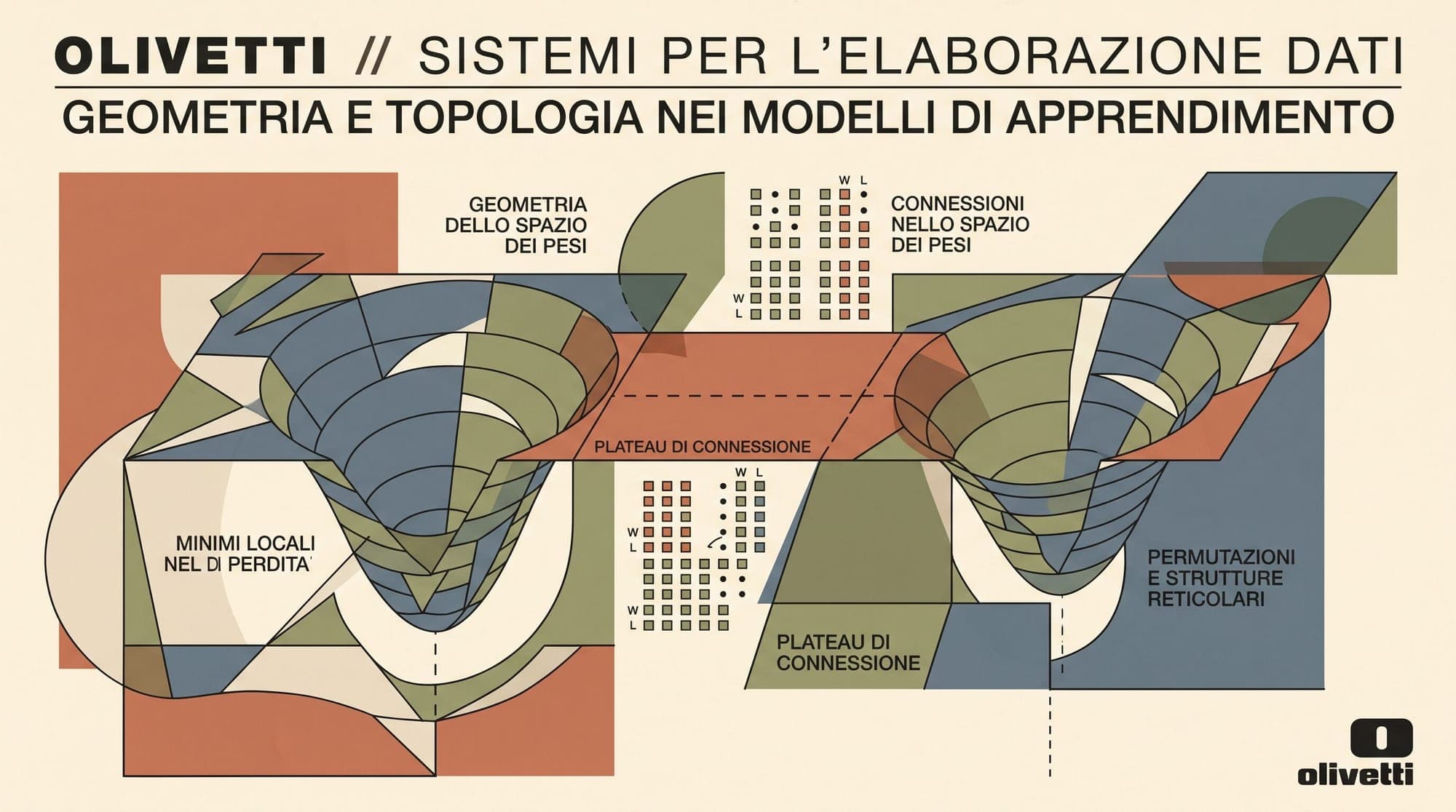
The classical intuition for high-dimensional optimization assumes that deep neural network loss landscapes are rugged, non-convex terrains populated by isolated local minima. Under this view, two models trained independently from distinct random initializations settle into distant, incompatible basins separated by insurmountable loss barriers. Direct parameter averaging between two such models typically degrades accuracy to random chance.

Research over the past several years has overturned this picture. Through the discovery of Linear Mode Connectivity (LMC) and the Single-Basin Conjecture, machine learning theorists have demonstrated that neural network optima are connected along continuous, low-loss valleys. When two models share a small initial optimization trajectory, or when their internal hidden representations are aligned to account for architectural permutation symmetries, the loss barrier between their weight configurations drops to zero.

Understanding Linear Mode Connectivity provides the theoretical foundation for critical techniques in modern foundation models, including model soups, task arithmetic, weight averaging, and decentralized asynchronous distributed training.

Linear Mode Connectivity and Permutation Alignment

The Geometry of Mode Connectivity

Mode connectivity describes the structural relationship between distinct minimizers of a loss objective $\mathcal{L}(\theta)$ over parameters $\theta \in \mathbb{R}^D$ .

Non-Linear Mode Connectivity

Before linear connectivity was formalized, Garipov et al. (2018) and Draxler et al. (2018) proved that local minima discovered by Stochastic Gradient Descent (SGD) are not isolated points. Instead, they are connected by continuous, non-linear paths of nearly constant low loss.

Given two local optima $\theta_A$ and $\theta_B$ , there exists a continuous parameterized curve $\phi(t): [0, 1] \to \mathbb{R}^D$ with $\phi(0) = \theta_A$ and $\phi(1) = \theta_B$ such that:

$\max_{t \in [0, 1]} \mathcal{L}(\phi(t)) \le \max(\mathcal{L}(\theta_A), \mathcal{L}(\theta_B)) + \epsilon$

These paths can be found using polygonal chains with a single bending point or piecewise Bézier curves. While non-linear connectivity demonstrated that loss surfaces are connected manifolds rather than disconnected basins, finding the connecting curve required explicit optimization along the path.

Linear Mode Connectivity and the Loss Barrier

Linear Mode Connectivity asks a stronger question: when is the simple straight-line segment connecting two parameter sets $\theta_A$ and $\theta_B$ free of loss barriers?

The linear interpolation between two models is parameterized by $\alpha \in [0, 1]$ :

$\theta(\alpha) = (1 - \alpha)\theta_A + \alpha \theta_B$

The loss barrier $\mathcal{B}(\theta_A, \theta_B)$ along this path measures the maximum excess error above the linear interpolation of the endpoint losses:

$\mathcal{B}(\theta_A, \theta_B) = \max_{\alpha \in [0, 1]} \left[ \mathcal{L}(\theta(\alpha)) - \left( (1 - \alpha)\mathcal{L}(\theta_A) + \alpha \mathcal{L}(\theta_B) \right) \right]$

Two models satisfy Linear Mode Connectivity if $\mathcal{B}(\theta_A, \theta_B) \le \epsilon$ , where $\epsilon$ is negligible relative to the baseline performance.

Early SGD Phase and the Lottery Ticket Hypothesis

In their investigation of the Lottery Ticket Hypothesis, Frankle, Dziugaite, Roy, and Carbin (2020) examined when during training networks become linearly connected.

If two networks are trained from different random seeds at step $0$ , interpolating their weights yields a massive loss barrier. However, if a single model is trained for $k$ initial steps of SGD, and then branched into two independent runs with different data ordering and SGD noise, the outcome shifts dramatically:

**Early Instability ($k < k^$):* The two branched models diverge into different optimization trajectories, resulting in a substantial loss barrier when interpolated.
**Linear Stability ($k \ge k^$):* After a critical threshold $k^*$ (often only a few hundred to a few thousand iterations), the two independently trained runs remain linearly mode connected ( $\mathcal{B} \approx 0$ ).

This finding demonstrated that SGD rapidly resolves the primary non-convex routing decisions in early training. Once the optimization enters a specific convex valley, SGD noise cannot knock the parameters out of that shared basin.

Permutation Symmetries and the Single-Basin Conjecture

While models branching from a shared checkpoint achieve LMC, models trained from completely independent random initializations ( $\theta_0^{(1)} \neq \theta_0^{(2)}$ ) still exhibited significant loss barriers.

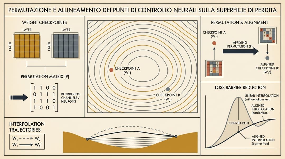
Researchers hypothesized that this barrier was not a fundamental property of the optimization landscape, but rather an artifact of permutation symmetries.

The Permutation Symmetry Group

In any multi-layer perceptron, convolutional network, or Transformer block, the ordering of hidden neurons or attention channels is arbitrary. Swapping two hidden units in layer $l$ and applying the inverse permutation to the incoming weights of layer $l+1$ leaves the input-output function of the network completely unchanged.

For a feedforward network with $L$ layers and hidden layer widths $d_1, d_2, \dots, d_{L-1}$ , the parameter space exhibits a discrete symmetry group of size:

$|\mathcal{G}| = \prod_{l=1}^{L-1} (d_l!)$

For even modest architectures, this represents an astronomically large number of functionally identical parameter configurations distributed across the loss landscape. If Model A converges to one permutation of hidden features and Model B converges to another, linearly interpolating their raw weights averages incompatible neurons together, creating destructive interference and catastrophic loss spikes.

The Entezari Conjecture

Entezari, Sedghi, Saukh, and Neyshabur (2021) formulated the Single-Basin Conjecture:

For sufficiently overparameterized neural networks, all minimizers found by standard SGD belong to a single connected basin modulo the permutation symmetry group $\mathcal{G}$ .

Formally, given two independently trained minimizers $\theta_A$ and $\theta_B$ , there exists a permutation $\pi \in \mathcal{G}$ acting on the hidden dimensions of $\theta_B$ such that:

$\mathcal{B}(\theta_A, \pi(\theta_B)) \approx 0$

Under this hypothesis, overparameterized neural networks do not possess millions of distinct, isolated minima. There is effectively only one global basin, replicated across permutations of the hidden unit coordinates.

Algorithmic Realization: Git Re-Basin

Finding the optimal permutation $\pi$ that aligns two networks in high-dimensional space is an NP-hard combinatorial assignment problem. Ainsworth, Hayase, and Srinivasa (2022) developed Git Re-Basin, introducing practical algorithms to search for matching permutations across layers.

Model A Checkpoint (θ_A) ──────────┐
                                   │
                                   ▼
Model B Checkpoint (θ_B) ──► [Neuron Permutation π] ──► [Weight Matching / REPAIR] ──► Zero-Barrier Interpolation: (1-α)θ_A + α π(θ_B)

Git Re-Basin explored three distinct matching paradigms:

1. Weight Matching

Weight matching seeks layer-wise permutation matrices $P_l \in \{0, 1\}^{d_l \times d_l}$ that minimize the Frobenius norm difference between the weight tensors of Model A and the permuted weight tensors of Model B:

$\min_{\{P_l\}_{l=1}^{L-1}} \sum_{l=1}^L \| W_l^A - P_l W_l^B P_{l-1}^T \|_F^2$

Because $P_0 = I$ (input features) and $P_L = I$ (output logits), the problem decomposes into coupled bipartite matching subproblems. Git Re-Basin solves this via coordinate ascent: iteratively fixing all permutations except $P_l$ , calculating the cost matrix $C_l = W_l^A (P_{l-1} W_l^B)^T + (W_{l+1}^A)^T P_{l+1} W_{l+1}^B$ , and solving the linear sum assignment problem via the Hungarian or Jonker-Volgenant algorithm.

2. Activation Matching

Rather than comparing static weights, activation matching computes the cross-covariance of intermediate representations across a calibration dataset $\mathcal{D}_{\text{calib}}$ .

For hidden layer $l$ , let $h_l^A(x) \in \mathbb{R}^{d_l}$ and $h_l^B(x) \in \mathbb{R}^{d_l}$ represent the post-activation vectors for input $x$ . The correlation matrix between neurons is:

$M_l(j, k) = \mathbb{E}_{x \sim \mathcal{D}_{\text{calib}}} \left[ h_{l, j}^A(x) \cdot h_{l, k}^B(x) \right]$

The optimal permutation $P_l$ is found by maximizing the trace $\text{Tr}(P_l M_l)$ , aligning neurons that perform identical functional transformations across the dataset.

3. Resolving Variance Collapse with REPAIR

Even when permutations align neurons correctly, linear interpolation can suffer from an activation variance mismatch. As observed by Jordan et al. (2022) in the REPAIR framework (Renormalizing Activations for Improving Re-basin), interpolating two independent sets of weights $(1-\alpha)W_A + \alpha \pi(W_B)$ reduces the variance of internal pre-activations:

$\text{Var}(z_{\alpha}) = (1 - \alpha)^2 \text{Var}(z_A) + \alpha^2 \text{Var}(z_B) + 2\alpha(1-\alpha)\text{Cov}(z_A, z_B)$

If the representations are not perfectly correlated ( $\text{Corr} < 1$ ), the intermediate activations shrink in magnitude, causing downstream layers to receive attenuated signals. REPAIR corrects this by computing the empirical mean and variance of activations across the interpolation path and rescaling batch normalization or LayerNorm running statistics accordingly.

Implications for Modern Foundation Models

Linear Mode Connectivity and permutation alignment are central to modern LLM pre-training, fine-tuning, and model management architectures.

Pre-Trained Base Model (θ_base)
         │
         ├──► Fine-Tune Task 1 ──► θ_1 (Task Vector τ_1 = θ_1 - θ_base)
         │
         ├──► Fine-Tune Task 2 ──► θ_2 (Task Vector τ_2 = θ_2 - θ_base)
         │
         ▼
Model Soup / Arithmetic Fusion:
θ_merged = θ_base + λ_1 τ_1 + λ_2 τ_2  (Linearly Connected, Zero Training Cost)

1. Model Soups and Weight Averaging

Wortsman et al. (2022) introduced Model Soups, demonstrating that fine-tuning a pre-trained base model with different hyperparameters, data orderings, or learning rates produces checkpoints that are naturally linearly mode connected.

Because all runs originate from the same pre-trained base checkpoint $\theta_{\text{base}}$ , they reside in the same low-loss basin. Averaging the weights of these fine-tuned models:

$\theta_{\text{soup}} = \frac{1}{M} \sum_{m=1}^M \theta_m$

consistently outperforms every individual model in accuracy, calibration, and out-of-distribution robustness without requiring any neuron permutation or inference-time ensemble overhead.

2. Task Arithmetic and Weight Merging

Techniques like Task Arithmetic (Ilharco et al., 2022), TIES-Merging (Yadav et al., 2023), and DARE (Yu et al., 2023) rely directly on Linear Mode Connectivity.

When distinct instruction-tuned or specialized models are adapted from a shared base LLM (e.g., LLaMA, Mistral, or Qwen), their parameter delta vectors $\tau_i = \theta_i - \theta_{\text{base}}$ form a linear vector space. Multi-task capabilities can be synthesized simply by computing linear combinations of task vectors:

$\theta_{\text{multi}} = \theta_{\text{base}} + \sum_{i=1}^K \lambda_i \tau_i$

Linear Mode Connectivity explains why these parameter combinations preserve factual knowledge and reasoning capabilities rather than collapsing the transformer's attention activations.

3. Distributed and Decentralized Training (DiLoCo)

In large-scale distributed pre-training across high-latency networks, synchronizing gradients at every step is bandwidth-prohibitive. Douillard et al. (2023) introduced DiLoCo (Distributed Low-Communication), where independent compute clusters run 500 or more inner optimization steps locally before synchronizing.

At each outer step, the master model performs an outer SGD update along the pseudo-gradient defined by the average parameter vector across workers. DiLoCo functions efficiently because overparameterized models initialized together maintain Linear Mode Connectivity over long inner optimization horizons.

Architectural Ceilings and Open Limits

While Linear Mode Connectivity holds robustly for fine-tuned checkpoints and moderately wide vision/language models, theoretical and practical limits remain:

| Regime | LMC Behavior | Primary Mechanism / Bottleneck | | :--- | :--- | :--- | | Shared Initialization Fine-Tuning | Zero barrier ( $\mathcal{B} \approx 0$ ) without alignment | Models remain in the initial pre-trained basin | | Wide Networks from Scratch | Near-zero barrier after permutation alignment | Git Re-Basin / Activation Matching | | Narrow / Deep Networks from Scratch | Residual loss barrier persists | Capacity limits; distinct topological paths | | Cross-Architecture Merging | Incompatible weight dimensions | Requires activation projection or adapter distillation |

Width vs. Depth Trade-Off: Entezari et al. (2021) and subsequent scaling studies proved that the permutation barrier decreases as layer width $d$ increases, but can worsen in extremely deep architectures with narrow bottlenecks. Overparameterized width is essential for creating redundant permutation paths.
Transformer Multi-Head Permutations: In multi-head attention mechanisms, permutation symmetries exist both across heads and within individual projection dimensions ( $W_q, W_k, W_v$ ). Aligning cross-attention circuits between independently pre-trained foundation models remains an active research challenge.
LayerNorm and RMSNorm Scale Drift: In transformer blocks without batch normalization, activation scaling during linear interpolation can interact non-linearly with RMSNorm layers, requiring explicit activation rescaling along the interpolation trajectory.

Summary

Linear Mode Connectivity and the Single-Basin Hypothesis redefine our understanding of neural network optimization:

Connected Basins: Neural network minima are not isolated pockets in weight space; they are connected along continuous, low-loss manifolds.
Early Basin Selection: SGD selects a convex loss valley during the earliest steps of training ( $k \ge k^*$ ), maintaining linear connectivity across different optimization paths.
Permutation Invariance: Apparent loss barriers between independently initialized models are largely artifacts of internal neuron permutations. Git Re-Basin algorithms align these symmetries to merge checkpoints directly.
Foundation Model Composability: LMC provides the formal mathematical underpinning for model soups, task arithmetic, and zero-cost model merging across modern foundation models.