Mixture-of-Depths (MoD): Mathematical Foundations, Dynamic Token-Level Compute Routing, Top-k Capacity Budgeting, and FLOP-Optimal Transformer Architectures

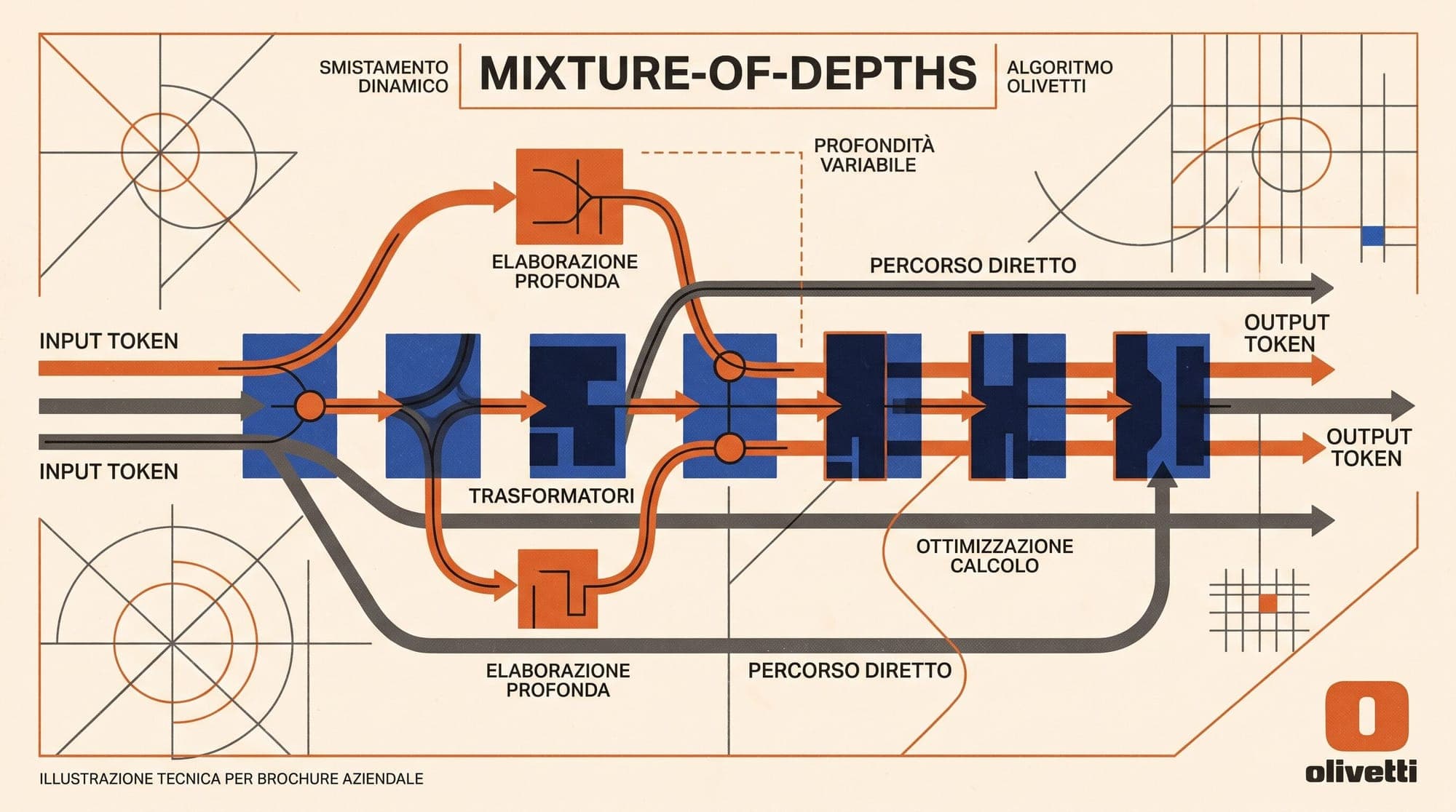
Standard autoregressive Transformers allocate an identical compute budget to every token in a sequence. Regardless of whether a token represents a trivial punctuation mark, a common grammatical function word, or a complex semantic reasoning step, the model applies the exact same sequence of multi-head self-attention and multilayer perceptron (MLP) operations across all $L$ layers.

In Mixture-of-Depths: Dynamically allocating compute in transformer-based language models, researchers at Google DeepMind (Raposo et al., 2024) introduced Mixture-of-Depths (MoD). MoD reallocates FLOPs dynamically across sequence positions and model depth. By enforcing an explicit total compute capacity per layer, MoD routes only a subset of informative tokens through attention and MLP blocks while allowing the remaining tokens to bypass computation entirely via residual skip connections.

Mathematical Formulation of Mixture-of-Depths

In a conventional Transformer layer $l$, the input tensor $X^l = [x_1^l, x_2^l, \dots, x_T^l]^T \in \mathbb{R}^{T \times d}$ undergoes computation across all $T$ token positions:

$$y_i^l = x_i^l + f_l(x_i^l)$$

where $f_l(\cdot)$ represents the computational block (multi-head attention or MLP) and $x_i^l \in \mathbb{R}^d$ is the hidden state vector at sequence position $i$.

Router Scoring and Dynamic Capacity Budgeting

Mixture-of-Depths introduces a learned router parameter vector $w_{r,l} \in \mathbb{R}^d$ at each routable layer $l$. The router assigns a scalar routing weight $r_i^l$ to each token position:

$$r_i^l = w_{r,l}^T x_i^l$$

Rather than applying a soft gating factor to all tokens or setting an unconstrained threshold (which creates variable tensor dimensions and destabilizes distributed hardware execution), MoD enforces a strict capacity factor $C \in (0, 1]$. The total number of tokens permitted to participate in computation block $f_l$ is bounded by capacity $k$:

$$k = \lfloor C \cdot T \rfloor$$

Typical configurations set $C = 0.5$ (50% token capacity) or $C = 0.125$ (12.5% token capacity). The layer determines the active token set $S_l$ by identifying the indices corresponding to the top-$k$ router scores:

$$S_l = \text{TopK}\left( \{r_i^l\}_{i=1}^T, k \right)$$

Block Execution and Residual Bypassing

Tokens belonging to index set $S_l$ are collected into a packed tensor $\tilde{X}^l \in \mathbb{R}^{k \times d}$ and processed through computation block $f_l$. The output of $f_l$ is scaled by the router weight $r_i^l$ to ensure continuous gradient flow during backpropagation:

$$y_i^l = \begin{cases} x_i^l + r_i^l \cdot f_l(x_i^l), & \text{if } i \in S_l \\ x_i^l, & \text{if } i \notin S_l \end{cases}$$

For tokens outside $S_l$, the computation block is omitted entirely. The hidden state propagates unchanged along the residual stream, incurring zero matrix multiply FLOPs for that layer.

Because the output is directly modulated by $r_i^l$, the loss gradient propagates to the router weights:

$$\frac{\partial \mathcal{L}}{\partial w_{r,l}} = \sum_{i \in S_l} \frac{\partial \mathcal{L}}{\partial y_i^l} f_l(x_i^l) (x_i^l)^T$$

This objective incentivizes the router to allocate high scores to tokens whose transformation under $f_l$ produces the greatest reduction in task loss.

Architectural Configurations and MoD Routing Schemes

MoD supports several routing topologies across Transformer layers:

1. Joint Attention and MLP Routing: A single router determines whether a token participates in both the self-attention block and the subsequent MLP block of layer $l$. Tokens bypassing the layer skip all compute primitives.
2. Staggered Block Routing: Independent routers gate self-attention and MLP sub-layers separately. A token may participate in self-attention to aggregate contextual information while bypassing the feed-forward projection, or vice versa.
3. Alternating Static and Dynamic Layers: Fixed dense Transformer layers alternate with MoD layers. This ensures periodic global information mixing across all sequence positions while saving compute in intermediate representations.

Mixture-of-Depths vs. Mixture-of-Experts (MoE)

While Mixture-of-Experts (Shazeer et al., 2017; DeepSeek AI, 2024) and Mixture-of-Depths both utilize conditional routing, their scaling dimensions differ:

• Mixture-of-Experts (MoE) routes tokens horizontally across parallel expert sub-networks. Total model parameter count expands significantly while compute per token remains constant.
• Mixture-of-Depths (MoD) routes tokens vertically through network depth. Total model parameter count remains constant while compute per token decreases according to capacity factor $C$.

Mixture-of-Depths-and-Experts (MoDE)

MoD and MoE can be integrated into a unified architecture termed MoDE. In MoDE, the routing mechanism selects both whether a token executes an MLP block (depth routing) and which specific expert MLP processes the token (expert routing).

This can be implemented by adding a null "no-op" path to a standard MoE top-$k$ router, or by cascading a binary MoD router ahead of an MoE expert gating network. MoDE enables models to decouple active parameters, total parameters, and sequence execution cost simultaneously.

Solving the Autoregressive Causal Routing Dilemma

During standard non-causal training and prefill phases, the top-$k$ selection operator evaluates router logits across all sequence positions $T$ simultaneously. However, during autoregressive generation (decoding), tokens are produced sequentially one token at a time. A token at position $t$ cannot rank its router score against future tokens $t+1, \dots, T$.

Raposo et al. evaluated two approaches to maintain causal autoregressive generation:

1. Auxiliary Binary Classification Loss

The primary router logits $r_i^l$ are supervised with an auxiliary binary cross-entropy loss $\mathcal{L}_{\text{aux}}$. The top-$k$ selections computed across the full sequence during training act as binary pseudo-labels:

$$\mathcal{L}_{\text{aux}} = -\frac{1}{T} \sum_{i=1}^T \left[ \mathbb{I}(i \in S_l) \log \sigma(r_i^l) + (1 - \mathbb{I}(i \in S_l)) \log(1 - \sigma(r_i^l)) \right]$$

where $\sigma(z) = \frac{1}{1 + e^{-z}}$. This loss shifts the router logits so that tokens destined for computation produce $\sigma(r_i^l) > 0.5$. During autoregressive decoding, the model routes token $t$ through block $f_l$ whenever $\sigma(r_t^l) > 0.5$, completely removing dependency on future tokens.

Empirical measurements demonstrate that this auxiliary objective achieves over 99% routing classification accuracy relative to true top-$k$ selection, while causing less than 0.3% degradation on the primary language modeling cross-entropy loss.

2. Predictor-Based Routing Modules

Alternatively, a small auxiliary MLP predictor processes intermediate hidden states from previous layers to forecast whether token $t$ warrants deep computation at layer $l$. Because the predictor relies exclusively on historical activations $x_{\le t}$, routing remains strictly causal at inference time.

IsoFLOP Scaling Analysis and Empirical Results

To evaluate whether dynamic compute allocation outperforms static scaling, Raposo et al. evaluated MoD models under compute-optimal training frameworks following the Chinchilla scaling laws (Hoffmann et al., 2022).

Under strict IsoFLOP comparisons (matching total training floating-point operations precisely across baselines and experimental models):

• Loss Parity with 50% Compute: An MoD Transformer configured with capacity factor $C = 0.5$ matches the validation loss of a standard dense Transformer while consuming 50% fewer FLOPs per forward pass in the routed layers.
• Superior IsoFLOP Performance: When trained with an identical total FLOP budget, an MoD model can be scaled to a larger baseline parameter footprint. The larger, sparsely routed model achieves lower validation loss and higher benchmark accuracy than the compute-optimal dense baseline.
• Inference Speedups: During generation, skipping 50% to 87.5% of layer computations reduces key-value (KV) cache memory access overhead and Tensor Core activation load, producing measurable latency reductions in high-throughput inference engines.

Hardware and Execution Mechanics

Deploying Mixture-of-Depths in production environments requires specific kernel handling to avoid hardware underutilization:

1. Static Shape Guarantees: Because capacity $k = \lfloor C \cdot T \rfloor$ is fixed prior to layer execution, memory allocation for intermediate activation buffers remains completely static. Unlike dynamic thresholding, MoD avoids GPU memory reallocation and tensor shape thrashing.
2. Gather/Scatter Overhead: Selected tokens must be gathered into contiguous memory blocks before entering high-performance fused GEMM and attention kernels (e.g., FlashAttention), and scattered back to the residual tensor afterward. Efficient CUDA implementations fuse index gathering into the input projection kernel to hide memory latency.
3. KV Cache Compression: For tokens that bypass self-attention layers, new key and value projections do not need to be written to GPU high-bandwidth memory (HBM). This reduces KV cache footprint for non-participating token positions.

Mixture-of-Depths demonstrates that the uniform FLOP allocation of standard Transformers is computationally inefficient. By combining explicit capacity budgets with learned routing, MoD provides a principled architectural mechanism for non-uniform compute distribution in large language models.

Sources

• Raposo, D., Ritter, S., Richards, B., Lillicrap, T., Humphreys, P. C., & Santoro, A. (2024). Mixture-of-Depths: Dynamically allocating compute in transformer-based language models. arXiv:2404.02258.
• Shazeer, N., Mirhoseini, A., Maziarz, K., Davis, A., Le, Q., Hinton, G., & Dean, J. (2017). Outrageously Large Neural Networks: The Sparsely-Gated Mixture-of-Experts Layer. arXiv:1701.06538.
• Hoffmann, J., Borgeaud, S., Mensch, A., Buchatskaya, E., Cai, T., Rutherford, E., Casas, D. de L., Hendricks, L. A., Welbl, J., Clark, A., Hennigan, T., Noland, J., Millican, K., Driessche, G. van den, Damoc, B., Guy, A., Osindero, S., Simonyan, K., Elsen, E., Rae, J. W., Vinyals, O., & Sifre, L. (2022). Training Compute-Optimal Large Language Models. arXiv:2203.15556.
• Dao, T., Fu, D. Y., Ermon, S., Rudra, A., & Ré, C. (2022). FlashAttention: Fast and Memory-Efficient Exact Attention with IO-Awareness. Advances in Neural Information Processing Systems (NeurIPS 2022).
• DeepSeek AI. (2024). DeepSeek-V2: A Strong, Economical, and Efficient Mixture-of-Experts Language Model. arXiv:2405.04434.