FlashAttention: Mathematical Foundations, Online Softmax Tiling, IO-Awareness, and Exact Attention Scaling

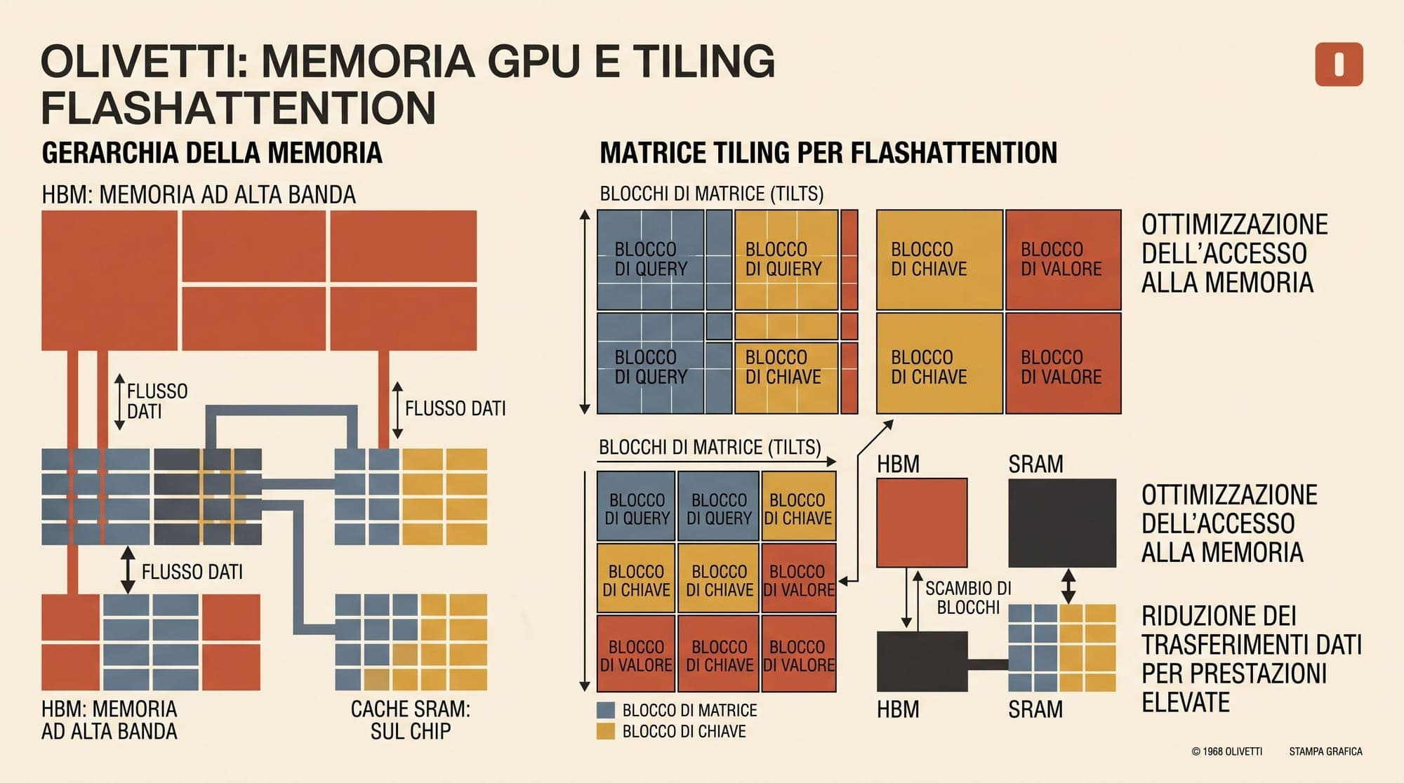
Standard multi-head self-attention in the Transformer architecture exhibits quadratic time and memory complexity with respect to sequence length $N$. While the $O(N^2)$ computational complexity is widely cited, the primary performance bottleneck in production hardware is not arithmetic throughput, but memory access overhead. On modern GPU architectures such as NVIDIA A100 and H100, tensor processing cores execute matrix multiplications at teraflop and petaflop scales, but memory bandwidth between High Bandwidth Memory (HBM) and on-chip SRAM remains the binding constraint.

Standard implementations of self-attention materialize the intermediate $N \times N$ attention score matrix and the subsequent softmax probability matrix in HBM. This causes excessive read and write traffic, reducing hardware utilization to a fraction of theoretical peak compute.

FlashAttention, introduced by Tri Dao et al. (2022), addresses this bottleneck through an IO-aware algorithm that computes exact attention without materializing the intermediate $N \times N$ matrices in global GPU memory. By leveraging online softmax normalization, SRAM block tiling, and selective activation recomputation in the backward pass, FlashAttention reduces memory accesses from quadratic $\Theta(N^2)$ to sub-quadratic $\Theta(N^2 d^2 / M)$, where $M$ is SRAM capacity and $d$ is head dimension. The resulting mechanism achieves 2x to 4x wall-clock speedups over standard attention while retaining exact mathematical equivalence. Subsequent iterations, including FlashAttention-2 and FlashAttention-3, further optimized work partitioning, warp-level scheduling, asynchronous memory transfers, and low-precision floating-point formats.

1. The Hardware Bottleneck: GPU Memory Hierarchies and Rooflines

To understand why standard attention scales poorly, one must evaluate the physical memory hierarchy of modern computing accelerators.

+-----------------------------------------------------------------------+
| GPU Global Memory (HBM3 / HBM2e)                                      |
| Capacity: 40 GB - 141 GB | Bandwidth: 1.5 TB/s - 4.8 TB/s            |
+-----------------------------------------------------------------------+
                                  |
                                  | High Latency / Limited Bandwidth
                                  v
+-----------------------------------------------------------------------+
| Streaming Multiprocessor (SM) On-Chip SRAM (Shared Memory / L1 Cache) |
| Capacity: 192 KB - 228 KB per SM | Bandwidth: ~19 TB/s aggregate      |
+-----------------------------------------------------------------------+
                                  |
                                  | Low Latency / Extremely High Bandwidth
                                  v
+-----------------------------------------------------------------------+
| Tensor Cores / Compute Registers                                      |
| Arithmetic Throughput: 312 TFLOPS (A100 FP16) - 1,979 TFLOPS (H100)   |
+-----------------------------------------------------------------------+

Memory Hierarchy Characteristics

A modern GPU divides memory into distinct tiers:

1. High Bandwidth Memory (HBM): Main device memory. It provides high capacity (for example, 80 GB on an A100 SXM4 or 141 GB on an H100 SXM5) but relatively constrained bandwidth (2.0 TB/s on A100; 3.35 TB/s on H100).
2. On-Chip Shared Memory / L1 Cache (SRAM): Located directly on each Streaming Multiprocessor (SM). An A100 contains 108 SMs with 192 KB of configurable shared memory per SM (approx. 20 MB total on-chip), delivering roughly 19 TB/s of aggregate bandwidth.
3. Register Files: The fastest memory, coupled directly to execution pipelines.

The Roofline Model and Arithmetic Intensity

Under the Roofline Model, an operation's attainable performance $P$ (FLOP/s) is bounded by:

$$P = \min\left(\text{Peak Arithmetic Throughput}, \, I \times \text{Peak Memory Bandwidth}\right)$$

where arithmetic intensity $I$ is defined as:

$$I = \frac{\text{Floating Point Operations (FLOPs)}}{\text{DRAM Bytes Transferred}}$$

For an NVIDIA A100 GPU running FP16 Tensor Core math:

• Peak Compute: 312 TFLOPS ($3.12 \times 10^{14}$ FLOP/s)
• Peak Memory Bandwidth: 2.0 TB/s ($2.0 \times 10^{12}$ B/s)
• Machine Balance / Threshold Intensity:

$$I_{\text{threshold}} = \frac{312 \times 10^{12}}{2.0 \times 10^{12}} = 156 \text{ FLOPs/Byte}$$

Any kernel with an arithmetic intensity below 156 FLOPs/byte on an A100 is memory-bandwidth bound.

Standard Self-Attention Memory Flow

Given input representations for queries $Q$, keys $K$, and values $V$ in $\mathbb{R}^{N \times d}$ (for sequence length $N$ and head dimension $d$), the standard attention computation follows:

$$S = Q K^T \in \mathbb{R}^{N \times N}$$

$$P = \text{softmax}(S) \in \mathbb{R}^{N \times N}$$

$$O = P V \in \mathbb{R}^{N \times d}$$

In standard PyTorch implementations:

1. Load $Q$ and $K$ from HBM, compute $S = QK^T$, and write $S$ of size $N^2$ back to HBM.
2. Load $S$ from HBM, compute $P = \text{softmax}(S)$, and write $P$ of size $N^2$ back to HBM.
3. Load $P$ and $V$ from HBM, compute $O = PV$, and write $O$ of size $N \times d$ back to HBM.

For sequence length $N = 4096$ and $d = 128$:

• Total FLOPs: $4 N^2 d = 4 \times 4096^2 \times 128 \approx 8.59 \times 10^9$ FLOPs.
• HBM Data Transferred (FP16): Loading and storing $S$ and $P$ ($4 \times N^2 \times 2$ bytes) plus loading $Q, K, V$ and storing $O$ ($8 \times N \times d \times 2$ bytes). The $N^2$ terms require $4 \times 16.78 \times 10^6 \times 2 \approx 134.2$ MB of HBM traffic.
• Arithmetic Intensity:

$$I_{\text{standard}} \approx \frac{8.59 \times 10^9 \text{ FLOPs}}{1.34 \times 10^8 \text{ Bytes}} \approx 64 \text{ FLOPs/Byte}$$

Because $64 \ll 156$, standard attention operates deep in the memory-bound regime. Most GPU execution cycles are spent stalling while waiting for DRAM transfers.

2. The Online Softmax Formulation

The key obstacle to computing attention entirely inside fast SRAM is the softmax operator. Given a vector $x \in \mathbb{R}^N$, the standard three-pass softmax requires global reduction:

$$m = \max_{1 \le j \le N} x_j$$

$$l = \sum_{j=1}^N e^{x_j - m}$$

$$\text{softmax}(x)_i = \frac{e^{x_i - m}}{l}$$

Computing $m$ and $l$ requires full visibility of all $N$ elements before any single output probability can be normalized. In naive block-based execution, this would necessitate writing intermediate scores to HBM between passes.

Derivation of the Incremental Online Normalizer

FlashAttention adopts the online softmax formulation established by Milakov and Gimelshein (2018) and Rabe and Staats (2021).

Suppose a row vector $x \in \mathbb{R}^N$ is partitioned into two contiguous blocks $x^{(1)} \in \mathbb{R}^{B}$ and $x^{(2)} \in \mathbb{R}^{B}$, such that $x = [x^{(1)}, x^{(2)}]$.

For block 1:

• Local maximum: $m^{(1)} = \max_j x_j^{(1)}$
• Local unnormalized sum: $l^{(1)} = \sum_j e^{x_j^{(1)} - m^{(1)}}$

When block 2 is loaded:

• Block maximum: $\tilde{m}^{(2)} = \max_j x_j^{(2)}$
• Block unnormalized sum: $\tilde{l}^{(2)} = \sum_j e^{x_j^{(2)} - \tilde{m}^{(2)}}$

The combined global maximum across both blocks is:

$$m^{(2)} = \max\left(m^{(1)}, \, \tilde{m}^{(2)}\right)$$

To combine the partition sums $l^{(1)}$ and $\tilde{l}^{(2)}$, they must be rescaled to the unified baseline $m^{(2)}$:

$$l^{(2)} = e^{m^{(1)} - m^{(2)}} l^{(1)} + e^{\tilde{m}^{(2)} - m^{(2)}} \tilde{l}^{(2)}$$

General Recurrence for Arbitrary Sequence Blocks

For a sequence partitioned into $T$ blocks $x^{(1)}, x^{(2)}, \dots, x^{(T)}$, the online recurrence maintains running statistics $(m^{(k)}, l^{(k)})$ at step $k$:

$$m^{(k)} = \max\left(m^{(k-1)}, \, \max_j x_j^{(k)}\right)$$

$$l^{(k)} = e^{m^{(k-1)} - m^{(k)}} l^{(k-1)} + \sum_j e^{x_j^{(k)} - m^{(k)}}$$

with base initializations $m^{(0)} = -\infty$ and $l^{(0)} = 0$.

Output Vector Update and Rescaling

The attention output for a single query row is $o = \sum_{j=1}^N P_j V_j = \frac{1}{l} \sum_{j=1}^N e^{x_j - m} V_j$.

Let $O^{(k-1)}$ be the unnormalized accumulator for the first $k-1$ blocks scaled to max $m^{(k-1)}$:

$$O^{(k-1)} = \sum_{j=1}^{(k-1)B} e^{x_j - m^{(k-1)}} V_j$$

When the $k$-th block of keys and values $(K^{(k)}, V^{(k)})$ is processed:

1. Compute local dot products: $S^{(k)} = q (K^{(k)})^T \in \mathbb{R}^B$
2. Find local block maximum: $\tilde{m}^{(k)} = \max_j S_j^{(k)}$
3. Update running maximum: $m^{(k)} = \max(m^{(k-1)}, \tilde{m}^{(k)})$
4. Compute unnormalized exponents for current block: $P^{(k)} = e^{S^{(k)} - m^{(k)}}$
5. Rescale previous accumulator and add new contribution:

$$O^{(k)} = e^{m^{(k-1)} - m^{(k)}} O^{(k-1)} + P^{(k)} V^{(k)}$$

1. Update normalizer:

$$l^{(k)} = e^{m^{(k-1)} - m^{(k)}} l^{(k-1)} + \sum_j P_j^{(k)}$$

After iterating through all $T$ blocks, the exact attention output vector is obtained by a single element-wise division:

$$O = \frac{O^{(T)}}{l^{(T)}}$$

This recurrence produces the exact same numerical result as standard softmax attention, without ever storing the full $N \times N$ score matrix.

3. FlashAttention Forward Algorithm and Tiling

The FlashAttention forward pass coordinates this online formulation across matrices $Q, K, V \in \mathbb{R}^{N \times d}$ loaded in SRAM-sized tiles.

+-----------------------------------------------------------------------------------+
| FlashAttention Forward Tiling Schema                                              |
+-----------------------------------------------------------------------------------+
  Query Blocks (Outer/Inner Loop): Tile size Br x d
  Key/Value Blocks: Tile size Bc x d

       K_1        K_2        K_3       ...       K_Tc
    +----------+----------+----------+        +----------+
    |  Bc x d  |  Bc x d  |  Bc x d  |        |  Bc x d  |
    +----------+----------+----------+        +----------+

 Q_1|  Tile S_11  Tile S_12  Tile S_13         Tile S_1Tc | -> O_1 (Br x d)
 Q_2|  Tile S_21  Tile S_22  Tile S_23         Tile S_2Tc | -> O_2 (Br x d)
 Q_3|  Tile S_31  Tile S_32  Tile S_33         Tile S_3Tc | -> O_3 (Br x d)
 ...|
Q_Tr|  Tile S_r1  Tile S_r2  Tile S_r3         Tile S_rTc | -> O_Tr (Br x d)

  Each SM loads Q_i into SRAM, then streams K_j, V_j blocks, updating
  running statistics (m_i, l_i) and accumulator O_i purely within SRAM.

Tile Size Selection

Given on-chip SRAM capacity $M$ (bytes), block dimensions $B_r$ (rows of $Q$) and $B_c$ (columns of $K, V$) are bounded by:

$$4 B_r d + 4 B_c d \le M$$

Typically, block sizes are configured as $B_r, B_c \in \{64, 128\}$ such that $Q_i, K_j, V_j$, local score tile $S_{ij} \in \mathbb{R}^{B_r \times B_c}$, and output accumulator $O_i \in \mathbb{R}^{B_r \times d}$ fit simultaneously in shared memory.

Step-by-Step Forward Pass Procedure

Input: Q, K, V in HBM (size N x d), SRAM capacity M.
Initialize: O = 0 in HBM (N x d), l = 0 in HBM (N), m = -inf in HBM (N).
Set tile dimensions: Bc = ceil(M / (4d)), Br = min(ceil(M / (4d)), d).
Divide Q into Tr = ceil(N / Br) blocks: Q_1, ..., Q_Tr.
Divide K, V into Tc = ceil(N / Bc) blocks: K_1, ..., K_Tc and V_1, ..., V_Tc.

For j = 1 to Tc:
    1. Load K_j, V_j from HBM into SRAM.
    For i = 1 to Tr:
        a. Load Q_i, O_i, l_i, m_i from HBM into SRAM.
        b. Compute S_ij = (Q_i K_j^T) / sqrt(d) in SRAM (size Br x Bc).
        c. Compute m_tilde_ij = rowmax(S_ij) in SRAM (size Br).
        d. Compute P_tilde_ij = exp(S_ij - m_tilde_ij) in SRAM (size Br x Bc).
        e. Compute l_tilde_ij = rowsum(P_tilde_ij) in SRAM (size Br).
        f. Compute new running max:
           m_i^new = max(m_i, m_tilde_ij)
        g. Compute new running normalizer:
           l_i^new = exp(m_i - m_i^new) * l_i + exp(m_tilde_ij - m_i^new) * l_tilde_ij
        h. Update output tile in SRAM:
           O_i = diag(exp(m_i - m_i^new)) * O_i + exp(m_tilde_ij - m_i^new) * (P_tilde_ij * V_j)
        i. Write m_i = m_i^new, l_i = l_i^new, and O_i back to HBM.

Final normalization: For each row i, compute O_i = diag(l_i)^(-1) * O_i in HBM.

4. Backward Pass and Selective Activation Recomputation

In standard backpropagation through attention, the forward pass must cache the entire attention probability matrix $P \in \mathbb{R}^{N \times N}$ in HBM so the backward pass can compute:

$$dV = P^T dO$$

$$dP = dO V^T$$

$$dS = P \circ \left( dP - \text{rowsum}(dP \circ P) \right)$$

$$dQ = \frac{1}{\sqrt{d}} dS K, \quad dK = \frac{1}{\sqrt{d}} dS^T Q$$

This caching requirement enforces an $O(N^2)$ memory footprint per attention head, causing out-of-memory (OOM) errors during long-sequence training.

Standard Attention Backward Pass:
Forward: Store P (N x N) in HBM -> Memory: O(N^2)
Backward: Load P (N x N) from HBM -> IO: O(N^2)

FlashAttention Backward Pass:
Forward: Store only m, l in HBM (size N) -> Memory: O(N)
Backward: Load Q_i, K_j from HBM, recompute S_ij and P_ij in SRAM on the fly -> IO: O(N^2 d^2 / M)

Recomputing Attention in SRAM

FlashAttention eliminates the $O(N^2)$ memory footprint by discarding $P$ after the forward pass. Instead, it only writes the normalization statistics $(m, l) \in \mathbb{R}^N$ to HBM, which scales linearly as $O(N)$.

During the backward pass:

1. Block tiles $Q_i, K_j, V_j$ and upstream gradient $dO_i$ are loaded into SRAM.
2. The score tile $S_{ij} = \frac{1}{\sqrt{d}} Q_i K_j^T$ is recomputed directly in SRAM.
3. Using cached values $m_i$ and $l_i$, the exact softmax probabilities are reconstructed:

$$P_{ij} = \text{diag}(l_i)^{-1} \exp\left(S_{ij} - m_i\right)$$

1. Gradients $dQ_i, dK_j, dV_j$ are computed entirely in SRAM and accumulated into HBM.

Gradient Derivation with Recomputed Statistics

Let $D_i = \text{rowsum}(dO_i \circ O_i) \in \mathbb{R}^{B_r}$. The gradient with respect to pre-softmax score matrix tile $S_{ij}$ simplifies to:

$$dS_{ij} = P_{ij} \circ \left( dO_i V_j^T - D_i \mathbf{1}^T \right)$$

By calculating $D_i$ prior to the inner loop over $K, V$ blocks, the kernel computes $dS_{ij}$ in SRAM without extra global memory transactions.

Recomputation Trade-Off Analysis

Although recomputing $S_{ij}$ in the backward pass adds $2 N^2 d$ FLOPs (a 33% increase in backward FLOP count), it completely removes $O(N^2)$ memory reads from HBM. Because the attention backward pass on GPUs is heavily memory-bound, eliminating HBM reads results in a net wall-clock speedup of 2x or more despite the extra arithmetic operations.

5. Algorithmic Evolution: FlashAttention-1, 2, and 3

The FlashAttention methodology has undergone three major architectural revisions to match evolving GPU hardware capabilities.

| Feature | FlashAttention-1 (2022) | FlashAttention-2 (2023) | FlashAttention-3 (2024) | | :--- | :--- | :--- | :--- | | Primary Target | NVIDIA Ampere (A100) | NVIDIA Ampere / Ada | NVIDIA Hopper (H100/H200) | | Outer Loop Dimension | $K, V$ blocks | $Q$ blocks | $Q$ blocks | | SM Parallelization | Batch, Heads | Batch, Heads, SeqLen ($Q$) | Batch, Heads, SeqLen ($Q$) | | SRAM Accumulator | Unscaled $O_i$ rescaled per step | Scaled by normalizer at end | Scaled by normalizer at end | | Hardware Specialization| Standard Tensor Cores | Optimized Warp Partitioning | TMA + WGMMA + FP8 Tensor Cores | | Asynchrony Model | Synchronous compute/load | Synchronous compute/load | Asynchronous ping-pong pipeline | | FP16 Peak Utilization | 30% - 40% on A100 | 50% - 73% on A100 | Up to 85% on H100 (840 TFLOPS) |

FlashAttention-2: Inverted Loops and Sequence Parallelism

FlashAttention-2 identified several hardware inefficiencies in the original algorithm:

1. Loop Inversion: FlashAttention-1 placed $K, V$ blocks in the outer loop and $Q$ blocks in the inner loop to save memory writes. However, this required frequent shared memory updates for $O_i$. FlashAttention-2 moves $Q$ to the outer loop and $K, V$ to the inner loop. An SM loads $Q_i$ once into registers and streams $K_j, V_j$ across it, keeping $O_i$ in registers until fully computed.
2. Parallelization Across Sequence Length: When batch size $\times$ number of heads is small (e.g., during long-context single-batch inference or multi-query attention), FlashAttention-1 underutilized GPU SMs. FlashAttention-2 parallelizes across the sequence length dimension of $Q$, ensuring all SMs remain saturated even for batch size 1.
3. Warp-Level Matrix Partitioning: In FlashAttention-1, warps within a thread block shared intermediate matrix multiplications, requiring synchronizations (__syncthreads()). FlashAttention-2 splits $Q_i$ across warps so each warp computes local GEMMs without cross-warp synchronization during the $Q K^T$ and $P V$ steps.

FlashAttention-3: Hopper Architecture and Asynchronous Pipelining

FlashAttention-3 targets the NVIDIA Hopper (H100) architecture, which introduced structural hardware primitives:

1. Tensor Memory Accelerator (TMA): A hardware engine that transfers multi-dimensional tensor blocks between global memory (HBM) and shared memory (SRAM) asynchronously without consuming SM instruction issues or register files.
2. Warp-Group Matrix Multiply and Accumulate (WGMMA): Instructions executed by a collective of four warps (128 threads) operating directly on shared memory matrices without register staging.
3. Warp Specialization: FlashAttention-3 partitions threads in a thread block into dedicated producer warps (issuing TMA loads) and consumer warps (executing WGMMA instructions), eliminating pipeline bubbles through circular shared-memory buffers.
4. Interleaved Softmax and Matmul: Hopper Tensor Cores and vector ALUs operate asynchronously. FlashAttention-3 overlaps the softmax exponentiation of block $j$ on the ALU with the matrix multiplication $Q K_{j+1}^T$ on the Tensor Cores.
5. Low-Precision FP8 Attention with Incoherent Processing: FP8 quantization introduces numerical instability in attention due to large outlier activations. FlashAttention-3 applies randomized Hadamard transformations ($Q \leftarrow Q H, K \leftarrow K H$) to spread activation energy across dimensions, preventing underflow/overflow in 8-bit formats and reaching 1.3 PFLOPS on H100.

6. Theoretical IO Complexity Bounds

The primary theoretical contribution of IO-aware attention is bounding memory access volume relative to SRAM size $M$.

Let $N$ be sequence length, $d$ be head dimension, and $M$ be SRAM capacity in elements, with $d \le M \le N d$.

Standard Attention IO Complexity

Standard attention writes and reads intermediate matrices $S, P \in \mathbb{R}^{N \times N}$ to HBM:

$$\text{IO}_{\text{standard}} = \Theta\left(N d + N^2\right) \text{ memory accesses}$$

For long sequences where $N \gg d$, IO complexity is dominated by $\Theta(N^2)$.

FlashAttention IO Complexity

In FlashAttention, $Q$ is split into $N / B_r$ blocks and $K, V$ into $N / B_c$ blocks, with $B_r, B_c \approx \Theta(M / d)$.

• Number of block pairs: $(N / B_r) \times (N / B_c) = \Theta\left(\frac{N^2 d^2}{M^2}\right)$.
• Data loaded per block pair: $O(B_r d + B_c d) = O(M)$.
• Total HBM memory accesses:

$$\text{IO}_{\text{Flash}} = \Theta\left( \frac{N^2 d^2}{M^2} \times M \right) = \Theta\left(\frac{N^2 d^2}{M}\right)$$

Lower Bound Optimality

Dao et al. proved via the Hong-Kung pebbling game that for any algorithm computing exact attention with SRAM of size $M$, the minimum number of HBM accesses is:

$$\Omega\left(\frac{N^2 d^2}{M}\right)$$

FlashAttention asymptotically matches this theoretical lower bound. The reduction factor in memory traffic relative to standard attention is:

$$\text{Speedup Factor} = \frac{\Theta(N^2)}{\Theta(N^2 d^2 / M)} = \Theta\left(\frac{M}{d^2}\right)$$

For typical parameters ($M \approx 10^5$ elements, $d = 128$), $M / d^2 \approx 6.1$, explaining the massive empirical reduction in DRAM traffic.

7. Systems Impact and Production Implementations

The development of IO-aware attention fundamentally reshaped modern LLM architectures, serving systems, and context window economics.

+-----------------------------------------------------------------------------------+
| Production Serving and Training Stack Integration                                |
+-----------------------------------------------------------------------------------+
| Large Language Models: Llama 3, DeepSeek-V3, Claude, GPT-4, Mistral               |
+-----------------------------------------------------------------------------------+
| Distributed Frameworks: Megatron-LM, DeepSpeed, PyTorch FSDP                      |
+-----------------------------------------------------------------------------------+
| Serving Engines: vLLM, SGLang, TensorRT-LLM, TGI                                 |
+-----------------------------------------------------------------------------------+
| Core Kernels: FlashAttention-2/3, FlashDecoding, PyTorch SDPA, CUTLASS            |
+-----------------------------------------------------------------------------------+

Context Length Scaling

Prior to FlashAttention, standard model context windows were constrained to 2,048 or 4,096 tokens (e.g., original GPT-3 and OPT). Storing the attention matrix for $N = 32,768$ across 32 layers and 32 heads in 16-bit precision would require:

$$\text{Memory} = 32 \times 32 \times 2 \times (32,768)^2 \text{ bytes} \approx 2.19 \text{ TB}$$

This rendered full-context training impossible without extreme tensor model parallelism. By reducing activation memory from $O(N^2)$ to $O(N)$ (storing only $m, l$), FlashAttention made 32K, 128K, and 1M+ context windows computationally tractable on standard GPU clusters.

FlashDecoding for Inference Prefill and Generation

During LLM autoregressive generation (decode phase), the query sequence length is $N_q = 1$, while the key-value sequence length $N_k$ grows with context history. Because $N_q = 1$, standard FlashAttention parallelization over $Q$ cannot utilize multiple SMs.

To address this, Flash-Decoding introduces parallelization across the $K, V$ sequence dimension:

1. The KV cache is split into $K$ chunks.
2. Each chunk computes partial attention outputs and running statistics $(m_k, l_k)$ in parallel across separate SMs using online softmax.
3. A final reduction kernel combines the $K$ partial outputs using the online softmax combination equations:

$$m = \max_k m_k, \quad l = \sum_k e^{m_k - m} l_k, \quad O = \sum_k \frac{e^{m_k - m} l_k}{l} O_k$$

This achieves near-constant generation latency as context length scales up to 64K tokens, eliminating the generation bottleneck in production inference engines like vLLM and SGLang.

Sources

• FlashAttention: Fast and Memory-Efficient Exact Attention with IO-Awareness (Dao et al., NeurIPS 2022)
• FlashAttention-2: Faster Attention with Better Parallelism and Work Partitioning (Dao, ICLR 2024)
• FlashAttention-3: Fast and Accurate Attention with Asynchrony and Low-precision (Shah et al., NeurIPS 2024)
• Online Normalizer Calculation for Softmax (Milakov & Gimelshein, 2018)
• Self-attention Does Not Need $O(n^2)$ Memory (Rabe & Staats, 2021)
• Attention Is All You Need (Vaswani et al., NeurIPS 2017)
• Roofline: An Insightful Visual Performance Model for Floating-Point Programs on Multicore Architectures (Williams et al., CACM 2009)
• Flash-Decoding for Fast Generation with Long Contexts (Dao et al., Stanford CRFM 2023)