Weight Pruning in Large Language Models: Mathematical Foundations of Magnitude Pruning, Wanda, SparseGPT, and Semi-Structured 2:4 Sparsity

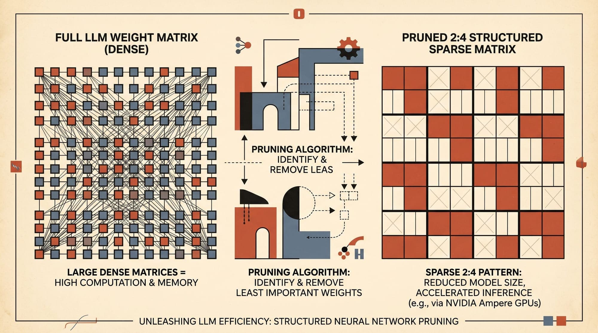
As frontier transformer models expand past hundreds of billions of parameters, model serving is constrained by memory capacity and memory bandwidth. In autoregressive token generation, memory bandwidth dominates latency because memory-bound matrix-vector operations require streaming entire weight matrices from High Bandwidth Memory (HBM) to on-chip SRAM for every single generated token.

Weight pruning reduces model size and memory bandwidth pressure by setting a fraction of weight parameters to zero. While classical pruning methods relied on iterative magnitude thresholding followed by extensive retraining, trillion-parameter foundation models cannot easily undergo compute-intensive fine-tuning cycles after compression. Modern post-training pruning techniques focus on one-shot, calibration-guided algorithms that sparsify models without backpropagation or parameter retraining.

The Mathematical Framework of Weight Pruning

Consider a single linear layer in a transformer network parameterized by weight matrix $W \in \mathbb{R}^{d_{\text{out}} \times d_{\text{in}}}$. Given an input activation tensor $X \in \mathbb{R}^{d_{\text{in}} \times N}$ collected over $N$ calibration tokens, the layer computes output $Y = W X$.

The goal of post-training weight pruning is to find a sparse weight matrix $\widehat{W}$ subject to a target sparsity constraint $s \in (0, 1)$ such that the layer output reconstruction error is minimized:

$$\min_{\widehat{W}} \| W X - \widehat{W} X \|_F^2 \quad \text{subject to} \quad \|\widehat{W}\|_0 \le (1 - s) \cdot \|W\|_0$$

where $\|\cdot\|_F$ denotes the Frobenius norm and $\|\cdot\|_0$ counts non-zero entries.

Second-Order Taylor Approximations: OBD and OBS

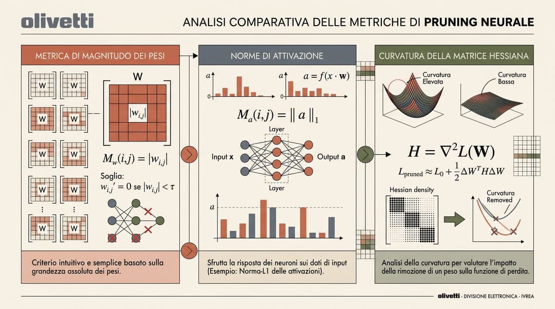
The foundation of analytical pruning traces to Optimal Brain Damage (LeCun et al., 1989) and Optimal Brain Surgeon (Hassibi and Stork, 1992). Expanding the loss function $\mathcal{L}(w)$ around an optimized parameter vector $w^*$ via Taylor expansion:

$$\Delta \mathcal{L} \approx g^T \Delta w + \frac{1}{2} \Delta w^T H \Delta w$$

where $g = \nabla_w \mathcal{L}(w^)$ is the gradient vector and $H = \nabla_w^2 \mathcal{L}(w^)$ is the Hessian matrix of second derivatives. Because pre-trained models reside near a local minimum, the first-order gradient $g \approx 0$, leaving the quadratic term $\frac{1}{2} \Delta w^T H \Delta w$.

When pruning parameter $w_q$ to zero ($\Delta w_q = -w_q$), Optimal Brain Damage assumes a diagonal Hessian, yielding the saliency score:

$$S_q^{\text{OBD}} = \frac{1}{2} H_{qq} w_q^2$$

Optimal Brain Surgeon removes the diagonal assumption. By solving the constrained optimization problem $\min_{\Delta w} \frac{1}{2} \Delta w^T H \Delta w$ subject to the constraint $e_q^T \Delta w + w_q = 0$, OBS derives both the optimal parameter removal score and the compensatory weight update for remaining unpruned parameters:

$$S_q^{\text{OBS}} = \frac{w_q^2}{2 [H^{-1}]_{qq}}$$

$$\Delta w = -\frac{w_q}{[H^{-1}]_{qq}} H^{-1} e_q$$

where $e_q$ is the standard basis vector with 1 at index $q$ and $[H^{-1}]_{qq}$ is the $q$-th diagonal element of the inverted Hessian matrix.

Magnitude Pruning and Its Breakdown in LLMs

Classical magnitude pruning ranks parameter importance purely by absolute magnitude:

$$S_{ij}^{\text{Mag}} = |W_{ij}|$$

In vision networks and smaller language models, magnitude pruning paired with iterative fine-tuning achieved high sparsity ratios. However, in modern decoder-only transformers (such as LLaMA, OPT, and BLOOM), one-shot magnitude pruning without retraining collapses perplexity at 20% to 30% sparsity.

The breakdown of magnitude pruning in large language models stems from emergent activation outliers. Research by Dettmers et al. (2022) revealed that once transformer models scale beyond 6.7 billion parameters, specific hidden dimensions develop activation magnitudes up to 100 times larger than average features. In linear transformations $Y_{i,:} = \sum_j W_{ij} X_{j,:}$, a weight $W_{ij}$ with small magnitude $|W_{ij}|$ paired with an outlier input channel $X_{j,:}$ contributes heavily to output activations. Magnitude pruning drops these small weights, destroying critical signal pathways.

Wanda: Pruning by Weights and Activations

To address the activation outlier bottleneck without computing expensive second-order derivatives, Sun et al. (2023) proposed Wanda (Pruning by Weights and activations).

Wanda evaluates weight saliency by scaling the absolute weight magnitude by the $\ell_2$-norm of the corresponding input activation column across calibration tokens:

$$S_{ij}^{\text{Wanda}} = |W_{ij}| \cdot \|X_{j,:}\|_2 = |W_{ij}| \cdot \sqrt{\sum_{k=1}^N X_{jk}^2}$$

Per-Output Row-Wise Comparison

Unlike global or whole-matrix sorting, Wanda evaluates pruning scores independently for each output channel (each row of $W$):

1. Compute input activation norms $\|X_{j,:}\|_2$ for all input features $j \in \{1, \dots, d_{\text{in}}\}$ over calibration samples.
2. Form the saliency matrix $S \in \mathbb{R}^{d_{\text{out}} \times d_{\text{in}}}$ where $S_{ij} = |W_{ij}| \cdot \|X_{j,:}\|_2$.
3. For each row $i \in \{1, \dots, d_{\text{out}}\}$, sort entries $S_{i,:}$ and set the lowest $s \times d_{\text{in}}$ elements to zero.

Wanda requires zero second-order Hessian inversions and zero parameter updates on remaining weights. Despite its simplicity, Wanda achieves 50% unstructured sparsity on LLaMA models with near-baseline perplexity, executing up to 300 times faster than full Hessian reconstruction methods.

SparseGPT: Large-Scale Second-Order Reconstruction

Frantar and Alistarh (2023) introduced SparseGPT, demonstrating that massive language models up to 175 billion parameters can be pruned to 50%–60% sparsity in one shot using exact second-order error compensation.

SparseGPT casts layer-wise pruning into a constrained least-squares problem over empirical activation covariance. For layer weights $W$ and calibration inputs $X$, the empirical Hessian is given by:

$$H = 2 X X^T + \lambda I$$

where $\lambda$ acts as a dampening factor to ensure numerical stability during matrix inversion.

Column-Wise Elimination and Batched Updates

Direct application of Optimal Brain Surgeon requires $\mathcal{O}(d_{\text{in}}^3)$ operations per pruned parameter, which is computationally intractable for matrices with $d_{\text{in}} = 8192$ or larger. SparseGPT reduces complexity through three architectural mechanics:

1. Cholesky Inversion: SparseGPT computes the inverse Hessian $H^{-1}$ once per layer using Cholesky factorization $H^{-1} = L^{-T} L^{-1}$.
2. Fixed Pruning Sequence: Parameters are evaluated column by column rather than searching globally across all remaining matrix entries.
3. Lazy Batched Updates: Weight updates are accumulated across blocks of columns (e.g., block size $B = 128$) and applied as matrix-matrix multiplications rather than sequential rank-1 updates.

When pruning column $j$, the optimal weight adjustment for unpruned columns $j' > j$ is computed as:

$$W_{:, j':d_{\text{in}}} \leftarrow W_{:, j':d_{\text{in}}} - \frac{W_{:, j} - \widehat{W}_{:, j}}{[H^{-1}]_{jj}} \cdot (H^{-1})_{j, j':d_{\text{in}}}$$

SparseGPT prunes 175B parameter models in under 4.5 hours on a single GPU while preserving downstream zero-shot accuracy.

Semi-Structured 2:4 Sparsity and Hardware Acceleration

While unstructured sparsity zeroes out arbitrary weights across the matrix, it produces random non-zero patterns that standard dense matrix multiplication hardware cannot accelerate efficiently without specialized sparse storage formats and sparse kernel overhead.

To bridge theoretical compression and real-world execution speed, modern GPU architectures (NVIDIA Ampere, Hopper, and Blackwell) implement native hardware support for semi-structured N:M sparsity, specifically 2:4 sparsity.

The 2:4 Sparsity Constraint

The 2:4 structured sparsity pattern mandates that for every contiguous block of 4 values along a row, exactly 2 values must be zero and 2 values remain non-zero (50% uniform sparsity):

$$\forall k \in \left\{1, \dots, \frac{d_{\text{in}}}{4}\right\}, \quad \|W_{i, 4k-3 : 4k}\|_0 \le 2$$

On Sparse Tensor Cores:

• The non-zero values are packed into a dense tensor of half the original width ($d_{\text{in}} / 2$).
• A compact metadata tensor stores 2-bit column indices per non-zero element to map positions during hardware execution.
• Matrix multiply units read half the memory bandwidth and execute double the arithmetic throughput, delivering up to a theoretical 2x speedup over dense operations.

Pruning Under N:M Constraints

Both Wanda and SparseGPT adapt directly to 2:4 structured constraints:

• 2:4 Wanda: In each 4-element block $W_{i, 4k-3:4k}$, evaluate scores $S_{i, 4k-3:4k} = |W_{i, 4k-3:4k}| \odot \|X_{4k-3:4k,:}\|_2$ and prune the two elements with smallest scores.
• 2:4 SparseGPT: In each 4-element block, select the two weights whose elimination minimizes the second-order reconstruction error, then apply OBS compensatory updates to all trailing columns.

Comparative Trade-Offs and Architectural Analysis

Understanding the trade-offs across pruning strategies guides deployment decisions in production inference pipelines:

• Unstructured Magnitude Pruning: Lowest compute overhead ($\mathcal{O}(1)$ per weight), but high perplexity degradation past 20% sparsity in LLMs due to activation outlier neglect.
• Wanda: Fast calibration pass ($\mathcal{O}(d_{\text{in}} \cdot N)$), accounts for activation outlier channels without matrix inversions, retains baseline accuracy up to 50% unstructured sparsity.
• SparseGPT: Second-order Hessian inversion ($\mathcal{O}(d_{\text{in}}^3 + d_{\text{out}} d_{\text{in}}^2)$), compensates remaining weights, achieves superior accuracy at higher sparsity ratios (60%+) and under strict 2:4 structured constraints.
• Hardware Acceleration: Unstructured sparsity primarily saves disk storage unless paired with specialized CPU/GPU sparse runtimes. In contrast, 2:4 semi-structured sparsity delivers direct inference latency speedups on NVIDIA Tensor Cores.

Sources

• LeCun, Y., Denker, J. S., & Solla, S. A. (1989). Optimal Brain Damage. Advances in Neural Information Processing Systems (NeurIPS 1989). https://proceedings.neurips.cc/paper/1989/file/6c340f25808812b26aaf40f1a0a83229-Paper.pdf
• Hassibi, B., & Stork, D. G. (1992). Second Order Derivatives for Network Pruning: Optimal Brain Surgeon. Advances in Neural Information Processing Systems (NeurIPS 1992). https://proceedings.neurips.cc/paper/1992/file/303ed4c69846ab36c2904d3ba8573050-Paper.pdf
• Frantar, E., & Alistarh, D. (2023). SparseGPT: Massive Language Models Can Be Accurately Pruned in One-Shot. Proceedings of the 40th International Conference on Machine Learning (ICML 2023). https://arxiv.org/abs/2301.00774
• Sun, M., Liu, Z., Bair, A., & Kolter, J. Z. (2023). A Simple and Effective Pruning Approach for Large Language Models. International Conference on Machine Learning (ICML 2023). https://arxiv.org/abs/2306.11695
• Mishra, A., Latorre, J. A., Pool, J., Stosic, D., Stosic, D., Venkatesh, G., Yu, C., & Micikevicius, P. (2021). Accelerating Sparse Deep Neural Networks. arXiv preprint. https://arxiv.org/abs/2104.08378
• Dettmers, T., Lewis, M., Belkada, Y., & Zettlemoyer, L. (2022). LLM.int8(): 8-bit Matrix Multiplication for Transformers at Scale. Advances in Neural Information Processing Systems (NeurIPS 2022). https://arxiv.org/abs/2208.07339