The Residual Stream in Transformers: How Linear Additive State, Subspace Projections, and Layer Accumulation Power Modern LLMs

In standard descriptions of transformer architectures, multi-head attention and feedforward networks receive the vast majority of analytical focus. However, the operational backbone coordinating these sublayers is the residual stream. First introduced in convolutional computer vision models by He et al. (2016) to mitigate vanishing gradients in deep networks, residual skip connections operate in large language models as a persistent, high-dimensional linear communication bus.

Rather than processing information sequentially through a rigid, monolithic transformation pipeline, modern transformers rely on the residual stream as a shared memory canvas. Individual attention heads and feedforward layers read specific features from this stream, perform isolated computations, and write additive updates back into the channel without destroying the existing state (Elhage et al., 2021). This linear additive formulation fundamentally dictates how transformer circuits compose, how representations scale with model depth, and how gradients propagate during optimization.

The Mathematical Mechanics: Reading and Writing to the Bus

At the start of a transformer forward pass, an input sequence of tokens is converted into initial continuous representations via a learned embedding matrix $W_E$ and combined with positional information:

$$x_0 = \text{Embed}(\text{tokens}) + \text{Pos}$$

The vector $x_0 \in \mathbb{R}^{d_{model}}$ enters the residual stream at layer 0. For each subsequent transformer layer $l \in \{1, \dots, L\}$, the state transitions according to two sequential additive operations:

$$x_l^{mid} = x_{l-1} + \text{Attn}_l(\text{LN}(x_{l-1}))$$

$$x_l = x_l^{mid} + \text{MLP}_l(\text{LN}(x_l^{mid}))$$

where $\text{LN}$ represents layer normalization (such as RMSNorm or standard Pre-LayerNorm).

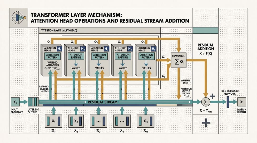
Every sublayer interacts with the residual stream through explicit linear projections:

1. Reading from the Stream: An attention head $h$ reads from the stream by projecting the unnormalized state via query, key, and value weights: $q = x W_Q^h$, $k = x W_K^h$, and $v = x W_V^h$. Similarly, a gated feedforward network (such as SwiGLU) reads the vector state via gate and up-projection matrices: $h_{gate} = x W_{gate}$ and $h_{up} = x W_{up}$.
2. Local Computation: The attention head calculates softmax attention patterns across sequence positions: $A = \text{softmax}(q k^T / \sqrt{d_k})$, producing intermediate value mixtures $r = A v$. The MLP evaluates non-linear activation gating: $m = \text{Swish}(h_{gate}) \odot h_{up}$.
3. Writing to the Stream: The computed representations are mapped back into the model dimension $d_{model}$ using output projection matrices $W_O^h$ and $W_{down}$. The resulting vectors are added directly into the stream:

$$\Delta x_l^{attn} = \sum_{h=1}^H r^h W_O^h, \quad \Delta x_l^{mlp} = m W_{down}$$

By expanding this recursion across all $L$ layers of the network, the final pre-unembedding state $x_L$ is revealed as a pure linear accumulation of updates:

$$x_L = x_0 + \sum_{l=1}^L \Delta x_l^{attn} + \sum_{l=1}^L \Delta x_l^{mlp}$$

Subspace Allocation and High-Dimensional Geometry

Because the residual stream is additive and fixed at width $d_{model}$ (such as 4,096 in LLaMA-7B or 8,192 in LLaMA-70B), the vector space acts as a shared memory address space. In high-dimensional Euclidean space, the number of mutually near-orthogonal directions scales exponentially with dimensionality.

This geometric property allows the transformer to partition the residual stream into quasi-independent linear subspaces (Elhage et al., 2021):

• Dedicated Feature Channels: A layer can write syntactic information (such as subject-verb number agreement) into subspace $S_1 \subset \mathbb{R}^{d_{model}}$, while another layer writes semantic domain tags into orthogonal subspace $S_2 \subset \mathbb{R}^{d_{model}}$. Because $S_1 \perp S_2$, operations projecting onto $S_1$ remain unaffected by updates written into $S_2$.
• Superposition and Polysemanticity: In practical LLMs, the number of distinct human concepts, grammatical rules, and factual associations vastly exceeds $d_{model}$. Models accommodate this by packing non-orthogonal features into superposition (Elhage et al., 2022), relying on non-linear MLP activations in subsequent layers to denoise and extract target signals when activated.

Direct Logit Attribution and Circuit Composition

The linear structure of the residual stream has critical implications for interpretability and model internals. In standard autoregressive architectures, the final prediction is obtained by projecting $x_L$ through an unembedding matrix $W_U \in \mathbb{R}^{d_{model} \times |V|}$:

$$\text{logits} = \text{LN}_{final}(x_L) W_U$$

Ignoring the final LayerNorm scale factor for first-order linear analysis, the logit vector decomposes additively across every component in the network:

$$\text{logits} \approx x_0 W_U + \sum_{l=1}^L \Delta x_l^{attn} W_U + \sum_{l=1}^L \Delta x_l^{mlp} W_U$$

This formulation enables Direct Logit Attribution (DLA). Researchers and engineers can compute $\Delta x_l^h W_U$ to measure the exact numerical contribution that a single attention head or MLP neuron makes toward promoting or suppressing a specific token in the vocabulary.

Furthermore, it explains how circuits compose across non-adjacent layers:

• K-Composition: An attention head in layer 10 can read key information directly written by layer 2 without layer 3 through 9 needing to forward or re-encode that information.
• V-Composition and Induction: Induction heads (Olsson et al., 2022) depend on previous-token heads writing position-shifted token identities into the stream, which downstream search heads subsequently attend to across long token spans.

Virtual Ensembles and Gradient Flow Dynamics

The additive skip connection fundamentally alters how depth functions in transformers. As demonstrated by Veit et al. (2016), residual networks do not behave like monolithic serial pipelines of depth $L$. Instead, an $L$-layer residual architecture acts as a virtual ensemble of $2^L$ distinct computational paths of varying lengths.

Input x0 ───────────────────────────────────────────────────────────> Output xL
   │                       │                       │                     ▲
   └──> [ Attn 1 ] ──(+)───┴──> [ Attn 2 ] ──(+)───┴──> [ MLP L ] ──(+)──┘
   │                  ▲    │                  ▲    │                 ▲
   └──> [ MLP 1 ] ────┘    └──> [ MLP 2 ] ────┘    └──> [ ... ] ─────┘

When evaluating a two-layer transformer block with paths through sublayers $\{f_1, f_2\}$, the computational graph unrolls into four parallel pathways:

$$x_2 = x_0 + f_1(x_0) + f_2(x_0) + f_2(f_1(x_0))$$

In an $L$-layer model, most data paths bypass the majority of intermediate layers, allowing the network to dynamically route tokens through shallow or deep computational circuits depending on task complexity.

Gradient Highway Mechanics

During backpropagation, the gradient of the loss $\mathcal{L}$ with respect to early representations $x_0$ is computed via the chain rule:

$$\frac{\partial \mathcal{L}}{\partial x_0} = \frac{\partial \mathcal{L}}{\partial x_L} \frac{\partial x_L}{\partial x_0} = \frac{\partial \mathcal{L}}{\partial x_L} \left( I + \sum_{l=1}^L \frac{\partial \Delta x_l}{\partial x_0} \right)$$

The presence of the identity matrix $I$ creates an uninterrupted gradient highway. Even if intermediate sublayer gradients $\frac{\partial \Delta x_l}{\partial x_0}$ vanish or become ill-conditioned, the backpropagated error signal flows directly to early layers and input embeddings without attenuation.

Architectural Trade-Offs and Stability Bottlenecks

While the residual stream provides modularity and stable optimization, scaling depth introduces physical and mathematical constraints:

Residual Stream Norm Growth in Pre-LN Models

In modern Pre-LN and Pre-RMSNorm transformers (Wang et al., 2019), each layer adds a zero-mean, non-zero variance update $\Delta x_l$ to $x_{l-1}$. Assuming updates are weakly correlated, the variance and Euclidean norm of the residual vector grow with depth:

$$\mathbb{E}[\|x_l\|_2^2] \approx \|x_0\|_2^2 + \sum_{i=1}^l \mathbb{E}[\|\Delta x_i\|_2^2] \sim \mathcal{O}(l)$$

Consequently, in deep models (such as 80 to 120 layers), $\|x_L\|_2$ is significantly larger than $\|x_0\|_2$. As the residual stream norm expands, the relative contribution of later layers $\frac{\|\Delta x_l\|}{\|x_l\|}$ naturally diminishes unless layer normalization rescales inputs or explicit branch scaling parameters (such as DeepNorm or ReZero multipliers $\alpha < 1$) are applied (Wang et al., 2022).

Bandwidth Bottlenecks in Deep-Narrow Configurations

Because every sublayer must communicate through $d_{model}$, narrow networks with extreme depth experience residual stream bandwidth pressure. If $d_{model}$ is too small relative to layer count $L$, sublayers overwrite or corrupt existing subspace allocations, degrading long-range circuit composition. Balancing residual width against depth remains a core optimization frontier in foundation model pre-training.

Sources

• A Mathematical Framework for Transformer Circuits (Elhage et al., 2021)
• Deep Residual Learning for Image Recognition (He et al., 2016)
• Residual Networks Behave Like Ensembles of Relatively Shallow Networks (Veit et al., 2016)
• Attention Is All You Need (Vaswani et al., 2017)
• In-context Learning and Induction Heads (Olsson et al., 2022)
• Toy Models of Superposition (Elhage et al., 2022)
• Learning Deep Transformer Models for Machine Translation (Wang et al., 2019)
• DeepNet: Scaling Transformers to 1,000 Layers (Wang et al., 2022)