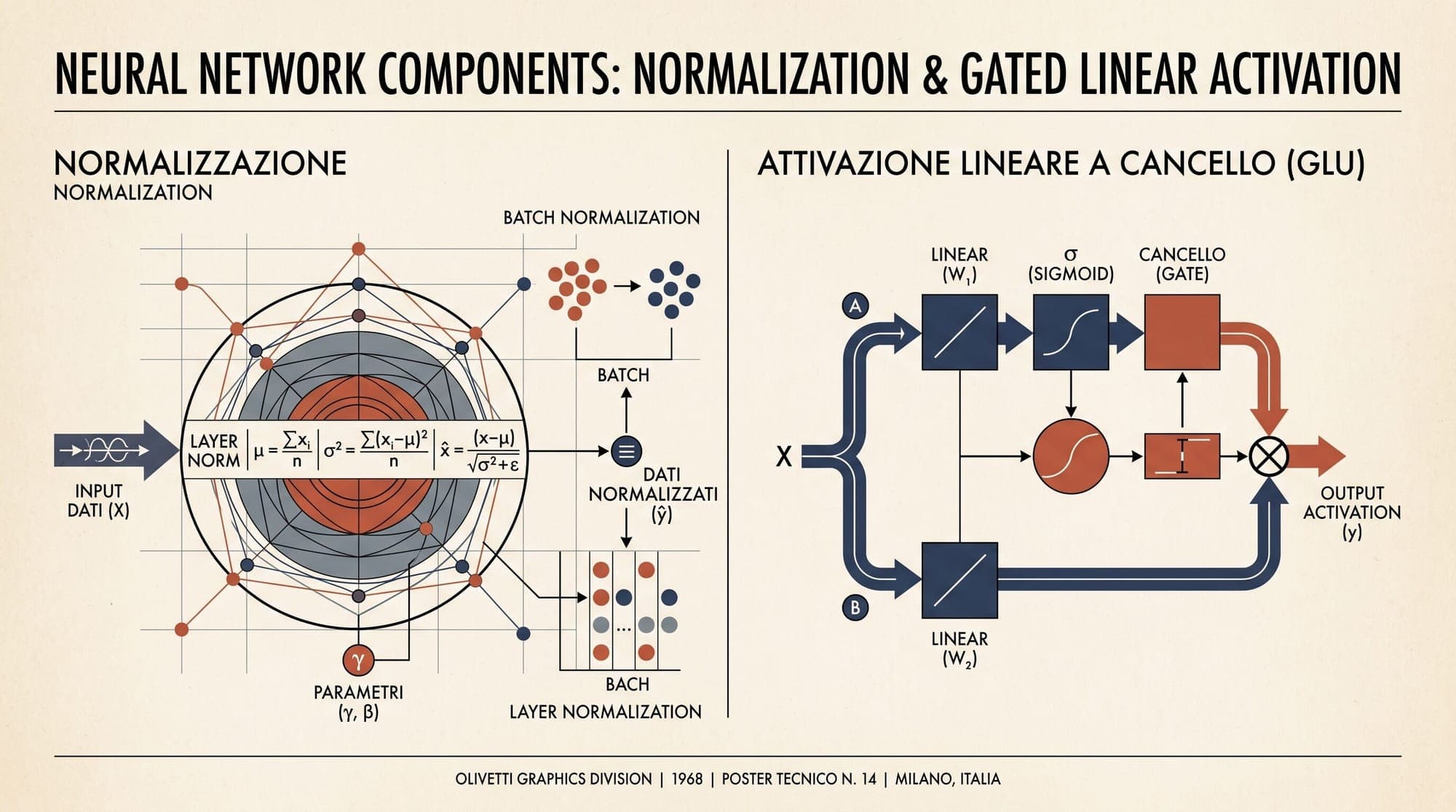
RMSNorm and SwiGLU: Mathematical Foundations of Scaling-Invariant Normalization, Gated Activations, and FFN Architectures in Modern LLMs

The architectural baseline of modern autoregressive large language models has converged on a distinct set of mathematical primitives. While early Transformer architectures relied on standard Layer Normalization, Post-LN residual routing, and two-layer Multi-Layer Perceptrons with ReLU or GELU activations, state-of-the-art open-weights models such as LLaMA, Mistral, Gemma, Qwen, and DeepSeek utilize a different combination: Root Mean Square Layer Normalization (RMSNorm), Pre-LN residual connections, and Gated Linear Unit feed-forward networks (specifically SwiGLU), typically implemented with zero additive bias parameters.

These architectural modifications are not arbitrary heuristic tweaks. They are mathematically grounded adjustments designed to optimize gradient propagation, reduce memory bandwidth overhead on modern GPU architectures, and increase the representational capacity of feed-forward layers at constant computational budgets.

Layer Normalization vs. RMSNorm: Mathematical Formulations

Standard Layer Normalization, introduced by Ba, Kiros, and Hinton (2016), normalizes activations across the feature dimension $d$ for each token vector $x \in \mathbb{R}^d$ . The standard formulation computes both the mean and variance across the hidden dimensions:

$\mu = \frac{1}{d} \sum_{i=1}^d x_i$

$\sigma = \sqrt{\frac{1}{d} \sum_{i=1}^d (x_i - \mu)^2 + \epsilon}$

$\hat{x} = \frac{x - \mu}{\sigma} \odot \gamma + \beta$

Here, $\gamma \in \mathbb{R}^d$ and $\beta \in \mathbb{R}^d$ are learnable scale (gain) and shift (bias) parameters, and $\epsilon > 0$ is a small numerical stabilizer.

The RMSNorm Formulation

In their analysis of Layer Normalization, Zhang and Sennrich (2019) investigated the theoretical components responsible for training stabilization in deep networks. They demonstrated that the computational benefit of LayerNorm stems almost entirely from scaling invariance rather than shift invariance (mean-centering).

RMSNorm replaces standard variance normalization with the root mean square statistic, discarding mean computation entirely:

$\text{RMS}(x) = \sqrt{\frac{1}{d} \sum_{i=1}^d x_i^2 + \epsilon}$

$\bar{x} = \frac{x}{\text{RMS}(x)} \odot \gamma$

In RMSNorm, the shift parameter $\beta$ is removed, leaving only the learnable gain parameter $\gamma \in \mathbb{R}^d$ .

LayerNorm:
  x ───> [ Compute Mean μ ] ───> [ Subtract Mean (x - μ) ] ───> [ Compute Variance σ² ] ───> [ Scale & Shift (γ, β) ] ───> Output

RMSNorm:
  x ───────────────────────────> [ Compute RMS(x) ] ──────────> [ Normalize & Scale (γ) ] ─────────────────────────> Output

Invariance Properties and Hardware Efficiency

LayerNorm provides two distinct invariance properties:

Shift invariance: $\text{LN}(x + c) = \text{LN}(x)$ for any constant offset scalar $c$ .
Scaling invariance: $\text{LN}(\alpha x) = \text{LN}(x)$ for any positive scaling scalar $\alpha > 0$ .

Zhang and Sennrich showed that the gradient regularization effect that prevents vanishing and exploding gradients in deep networks is governed by the scaling invariance property. Shift invariance has negligible impact on training dynamics across deep Transformer models.

Removing the mean computation provides significant advantages for GPU kernel execution:

Elimination of redundant reduction passes: Standard LayerNorm requires two reduction passes across the hidden dimension (one to calculate the mean $\mu$ , and a second to calculate the variance $\sigma^2$ ). RMSNorm requires only a single reduction pass to compute the sum of squares.
Memory bandwidth reduction: In fused CUDA and Triton kernels, avoiding the intermediate subtraction pass reduces registers per thread and minimizes SRAM/HBM round trips. This delivers a 10% to 50% execution speedup for the normalization kernel itself, which directly impacts training and inference throughput since normalization executes twice per Transformer block.

Normalization Placement: Pre-LN and Gradient Stability

The placement of normalization layers relative to the residual stream dictates gradient propagation through deep networks.

Post-LN Dynamics

The original Transformer architecture by Vaswani et al. (2017) placed normalization after the residual addition:

$x_{l+1} = \text{Norm}(x_l + \text{SubLayer}(x_l))$

In Post-LN architectures, the gradient backpropagated from layer $L$ to layer $l$ is scaled by the product of normalization derivatives across all intermediate layers:

$\frac{\partial x_L}{\partial x_l} = \prod_{k=l}^{L-1} \left( \frac{\partial \text{Norm}(z_k)}{\partial z_k} \left( I + \frac{\partial \text{SubLayer}(x_k)}{\partial x_k} \right) \right)$

As network depth increases, the normalization gradient scaling causes vanishing gradients in early layers during initialization. Consequently, Post-LN models require carefully tuned learning rate warmup schedules to prevent optimization divergence.

Pre-LN and the Identity Highway

Modern LLMs universally adopt Pre-LN (specifically Pre-RMSNorm):

$x_{l+1} = x_l + \text{SubLayer}(\text{RMSNorm}(x_l))$

By placing RMSNorm on the branch of the sublayer before the transformation, the residual connection forms an unobstructed identity path:

$\frac{\partial x_L}{\partial x_l} = I + \sum_{k=l}^{L-1} \frac{\partial \text{SubLayer}(\text{RMSNorm}(x_k))}{\partial x_l}$

The leading identity term $I$ ensures that gradients flow back to early layers without attenuation or explosion, allowing stable training of models with 100+ layers without delicate warmup dependencies.

Feed-Forward Networks: From Standard MLPs to Gated Linear Units

In standard Transformer architectures, the feed-forward network (FFN) consists of two linear projections with an element-wise non-linear activation function in between:

$\text{FFN}_{\text{Standard}}(x) = \sigma(x W_1 + b_1) W_2 + b_2$

Where $W_1 \in \mathbb{R}^{d_{\text{model}} \times d_{\text{ff}}}$ , $W_2 \in \mathbb{R}^{d_{\text{ff}} \times d_{\text{model}}}$ , and $\sigma$ is typically ReLU or Gaussian Error Linear Unit (GELU), as introduced by Hendrycks and Gimpel (2016). Standard configurations set $d_{\text{ff}} = 4 d_{\text{model}}$ , yielding a parameter count of $8 d_{\text{model}}^2$ (ignoring bias vectors).

Gated Linear Units (GLU)

Dauphin et al. (2016) introduced Gated Linear Units for sequence modeling in convolutional networks. A GLU replaces the static activation function with a component-wise product of two distinct linear projections, one of which is modulated by a gating function:

$\text{GLU}(x, W, V) = \sigma(x W) \otimes (x V)$

Where $\otimes$ denotes element-wise (Hadamard) multiplication, $W$ is the gating projection, and $V$ is the value (or up) projection.

Shazeer's GLU Variants: ReGLU, GEGLU, and SwiGLU

Noam Shazeer (2020) extended the GLU formulation to Transformer feed-forward sublayers by exploring different non-linear activation functions in place of the standard sigmoid $\sigma$ :

$\text{ReGLU}(x, W, V) = \max(0, x W) \otimes (x V)$

$\text{GEGLU}(x, W, V) = \text{GELU}(x W) \otimes (x V)$

$\text{SwiGLU}(x, W, V, \beta) = \text{Swish}_\beta(x W) \otimes (x V)$

The Swish activation function, identified by Ramachandran, Zoph, and Le (2017) via automated search (also known as the Sigmoid Linear Unit or SiLU when $\beta=1$ ), is defined as:

$\text{Swish}_\beta(z) = z \cdot \text{sigmoid}(\beta z) = \frac{z}{1 + e^{-\beta z}}$

For modern LLM implementations, $\beta = 1$ is standard, reducing the activation to $\text{SiLU}(z) = z \cdot \sigma(z)$ .

The complete SwiGLU feed-forward layer consists of three linear transformations:

$\text{FFN}_{\text{SwiGLU}}(x) = \left( \text{SiLU}(x W_{\text{gate}}) \odot (x W_{\text{up}}) \right) W_{\text{down}}$

Where:

$W_{\text{gate}} \in \mathbb{R}^{d_{\text{model}} \times d_{\text{ff}}}$ projects the input into the gating path.
$W_{\text{up}} \in \mathbb{R}^{d_{\text{model}} \times d_{\text{ff}}}$ projects the input into the value path.
$W_{\text{down}} \in \mathbb{R}^{d_{\text{ff}} \times d_{\text{model}}}$ projects the gated intermediate representation back to the model hidden dimension.

Parameter Balancing and Dimensioning

A standard two-matrix FFN with hidden dimension $d_{\text{ff\_std}} = 4 d_{\text{model}}$ contains:

$\text{Params}_{\text{Standard}} = 2 \cdot d_{\text{model}} \cdot d_{\text{ff\_std}} = 8 d_{\text{model}}^2$

Because SwiGLU introduces a third weight matrix ( $W_{\text{gate}}$ , $W_{\text{up}}$ , and $W_{\text{down}}$ ), the total parameter count for a hidden dimension $d_{\text{ff}}$ becomes:

$\text{Params}_{\text{SwiGLU}} = 3 \cdot d_{\text{model}} \cdot d_{\text{ff}}$

To keep the computational and parameter cost equivalent to a standard $4 d_{\text{model}}$ FFN, the intermediate dimension $d_{\text{ff}}$ must be adjusted:

$3 \cdot d_{\text{model}} \cdot d_{\text{ff}} = 8 d_{\text{model}}^2 \implies d_{\text{ff}} = \frac{8}{3} d_{\text{model}} \approx 2.667 d_{\text{model}}$

Hardware-Aligned Dimensioning in Production

In production architectures such as Meta's LLaMA series (Touvron et al., 2023), $d_{\text{ff}}$ is calculated using the $\frac{8}{3} d_{\text{model}}$ ratio and subsequently rounded up to a multiple of 256 or 64.

This rounding ensures that matrix dimensions align with the warp tile dimensions of NVIDIA Tensor Cores (such as $16 \times 16 \times 16$ or $16 \times 8 \times 32$ MMA operations), preventing execution divergence and padding overhead in matrix multiplications:

$d_{\text{ff}} = 256 \cdot \left\lceil \frac{\frac{8}{3} d_{\text{model}}}{256} \right\rceil$

For example, in a model with $d_{\text{model}} = 4096$ , the theoretical $\frac{8}{3} d_{\text{model}}$ is approximately $10922.67$ . Rounding to the nearest multiple of 256 yields $d_{\text{ff}} = 11008$ . Some configurations (such as LLaMA-3 8B) scale $d_{\text{ff}}$ even higher to $14336$ (a $\approx 3.5 d_{\text{model}}$ ratio) to allocate higher parameter capacity to the FFN sublayers while keeping attention parameter footprints fixed.

Why SwiGLU Outperforms Traditional Activations

Empirical benchmarks across large-scale pre-training runs consistently show that SwiGLU achieves lower validation perplexity than ReLU, GELU, and classical GLU at equivalent compute budgets. Several mathematical characteristics explain this performance advantage:

1. Dynamic Multiplicative Gating

In standard FFNs, activation functions apply a static scalar non-linearity to each channel independently: $y_i = \sigma(z_i)$ . In SwiGLU, the value projection $x W_{\text{up}}$ is dynamically scaled by $\text{SiLU}(x W_{\text{gate}})$ . The gating vector acts as a continuous, input-dependent filter that can selectively suppress or amplify specific feature channels based on context.

2. Smooth, Non-Monotonic Gradient Landscape

The SiLU activation function is smooth and non-monotonic:

$\text{SiLU}(z) = \frac{z}{1 + e^{-z}}$

Its first derivative with respect to $z$ is:

$\frac{d}{dz}\text{SiLU}(z) = \sigma(z) + z \sigma(z)(1 - \sigma(z)) = \sigma(z) \left( 1 + z(1 - \sigma(z)) \right)$

For positive values ( $z \gg 0$ ), $\frac{d}{dz}\text{SiLU}(z) \approx 1$ . For large negative values ( $z \ll 0$ ), $\frac{d}{dz}\text{SiLU}(z) \approx 0$ . Crucially, for moderately negative values (near $z \approx -1.28$ ), SiLU dips slightly below zero to a minimum of approximately $-0.278$ , and its derivative is non-zero.

Unlike ReLU, which has a hard zero derivative for all negative inputs (leading to irreversible neuron death during training), SiLU allows small gradient signals to propagate back through negative pre-activations, preserving optimization flexibility.

Activation Value Comparison:
  z = -3.0  --> ReLU(z) = 0.000, GELU(z) ≈ -0.004, SiLU(z) ≈ -0.142
  z = -1.0  --> ReLU(z) = 0.000, GELU(z) ≈ -0.159, SiLU(z) ≈ -0.269
  z =  0.0  --> ReLU(z) = 0.000, GELU(z) =  0.000, SiLU(z) =  0.000
  z =  1.0  --> ReLU(z) = 1.000, GELU(z) ≈  0.841, SiLU(z) ≈  0.731
  z =  3.0  --> ReLU(z) = 3.000, GELU(z) ≈  2.996, SiLU(z) ≈  2.858

3. Bilinear Higher-Order Interactions

The product $\text{SiLU}(x W_{\text{gate}}) \odot (x W_{\text{up}})$ introduces quadratic interaction terms between the linear projections of $x$ . A single SwiGLU layer can compute second-order polynomial combinations of input features, providing significantly richer representational capacity than standard affine transformations followed by univariate non-linearities.

Elimination of Additive Bias Parameters

A complementary trend across modern architectures (LLaMA, Mistral, Gemma 2, Qwen2.5) is the complete removal of additive bias terms ( $b = 0$ ) across all projection matrices and normalization layers:

Attention projections: $Q = x W_Q, \quad K = x W_K, \quad V = x W_V, \quad O = \text{Attn} \cdot W_O$
SwiGLU projections: $\text{Gate} = x W_{\text{gate}}, \quad \text{Up} = x W_{\text{up}}, \quad \text{Down} = \text{Inter} \cdot W_{\text{down}}$
Normalization: $y = \frac{x}{\text{RMS}(x)} \odot \gamma$

Eliminating bias terms provides three concrete benefits:

Memory overhead: Reduces optimizer state memory (e.g., in AdamW, each parameter requires 8 additional bytes for first and second moments).
Quantization stability: Additive biases frequently accumulate systematic offset errors during low-precision post-training quantization (such as FP8, INT8, and INT4 weight-only schemes). Zero-bias matrices produce activation distributions centered around zero, reducing asymmetric clipping errors.
Long-context extrapolation: Bias terms in linear projections can cause hidden state magnitudes to drift monotonically as sequence lengths scale into tens of thousands of tokens.

PyTorch Reference Implementation

The following module implements Pre-RMSNorm and a zero-bias SwiGLU feed-forward layer compatible with modern open-weights architectures:

import torch
import torch.nn as nn
import torch.nn.functional as F

class RMSNorm(nn.Module):
    """
    Root Mean Square Layer Normalization (RMSNorm).
    Reference: Zhang & Sennrich (2019) - https://arxiv.org/abs/1910.07467
    """
    def __init__(self, dim: int, eps: float = 1e-6):
        super().__init__()
        self.eps = eps
        self.weight = nn.Parameter(torch.ones(dim))

    def _norm(self, x: torch.Tensor) -> torch.Tensor:
        # Compute root mean square along the last dimension
        return x * torch.rsqrt(x.pow(2).mean(-1, keepdim=True) + self.eps)

    def forward(self, x: torch.Tensor) -> torch.Tensor:
        output = self._norm(x.float()).type_as(x)
        return output * self.weight

class SwiGLUFeedForward(nn.Module):
    """
    SwiGLU Feed-Forward Network with zero-bias linear projections.
    Reference: Shazeer (2020) - https://arxiv.org/abs/2002.05202
    """
    def __init__(self, d_model: int, d_ff: int | None = None, multiple_of: int = 256):
        super().__init__()
        # If d_ff is not provided, calculate 8/3 * d_model rounded to multiple_of
        if d_ff is None:
            d_ff = int(2 * (4 * d_model) / 3)
            d_ff = multiple_of * ((d_ff + multiple_of - 1) // multiple_of)

        self.w_gate = nn.Linear(d_model, d_ff, bias=False)
        self.w_up = nn.Linear(d_model, d_ff, bias=False)
        self.w_down = nn.Linear(d_ff, d_model, bias=False)

    def forward(self, x: torch.Tensor) -> torch.Tensor:
        # SwiGLU: (SiLU(x * W_gate) * (x * W_up)) * W_down
        return self.w_down(F.silu(self.w_gate(x)) * self.w_up(x))

class TransformerBlock(nn.Module):
    """
    Pre-RMSNorm Transformer Block with SwiGLU FFN.
    """
    def __init__(self, d_model: int, num_heads: int):
        super().__init__()
        self.attention_norm = RMSNorm(d_model)
        self.attention = nn.MultiheadAttention(d_model, num_heads, bias=False, batch_first=True)
        self.ffn_norm = RMSNorm(d_model)
        self.ffn = SwiGLUFeedForward(d_model)

    def forward(self, x: torch.Tensor) -> torch.Tensor:
        # Pre-LN Attention residual branch
        normed_attn_in = self.attention_norm(x)
        attn_out, _ = self.attention(normed_attn_in, normed_attn_in, normed_attn_in)
        x = x + attn_out

        # Pre-LN SwiGLU residual branch
        x = x + self.ffn(self.ffn_norm(x))
        return x

Summary Comparison

The shift from first-generation Transformer layers to modern architectural primitives is summarized below:

Normalization algorithm: LayerNorm (with mean subtraction and variance normalization) replaced by RMSNorm (scaling by root mean square alone).
Normalization parameters: Scale $\gamma$ and shift $\beta$ replaced by scale $\gamma$ only.
Normalization topology: Post-LN replaced by Pre-LN to maintain an unattenuated identity gradient highway.
FFN activation function: ReLU / GELU replaced by SwiGLU ( $\text{SiLU}(x W_{\text{gate}}) \odot x W_{\text{up}}$ ).
FFN projection count: 2 matrices ( $W_1, W_2$ ) replaced by 3 matrices ( $W_{\text{gate}}, W_{\text{up}}, W_{\text{down}}$ ).
Intermediate FFN dimension: $4 d_{\text{model}}$ adjusted to $\frac{8}{3} d_{\text{model}}$ (rounded to multiples of 256) to maintain parameter parity.
Bias parameters: Explicit bias vectors across attention, FFN, and normalization removed ( $b = 0$ ).