Grouped-Query Attention (GQA) and Multi-Query Attention (MQA): Mathematical Foundations, Arithmetic Intensity, and KV-Cache Scaling Mechanics

Autoregressive large language model inference is governed by a fundamental hardware asymmetry. During the initial prompt processing phase (prefill), computation is compute-bound because matrix multiplications process entire sequences in parallel. During sequential token generation (decoding), execution becomes strictly memory-bandwidth bound. For each generated token, the accelerator must transfer the entire model weight matrix and the accumulated Key-Value (KV) cache from High Bandwidth Memory (HBM) to on-chip SRAM to execute a single token step.

In standard Multi-Head Attention (MHA), introduced by Vaswani et al. (2017), the number of key-value projection heads equals the number of query heads ($H_Q = H_K = H_V = H$). As sequence lengths expand into tens of thousands of tokens and concurrent batch sizes scale, the memory footprint and bandwidth consumption of the KV cache dominate total serving costs.

To resolve this memory bottleneck, two architectural variants alter the projection dimensionality of keys and values:

1. Multi-Query Attention (MQA), introduced by Shazeer (2019), which collapses the key and value heads into a single shared head ($H_K = H_V = 1$) across all query heads.
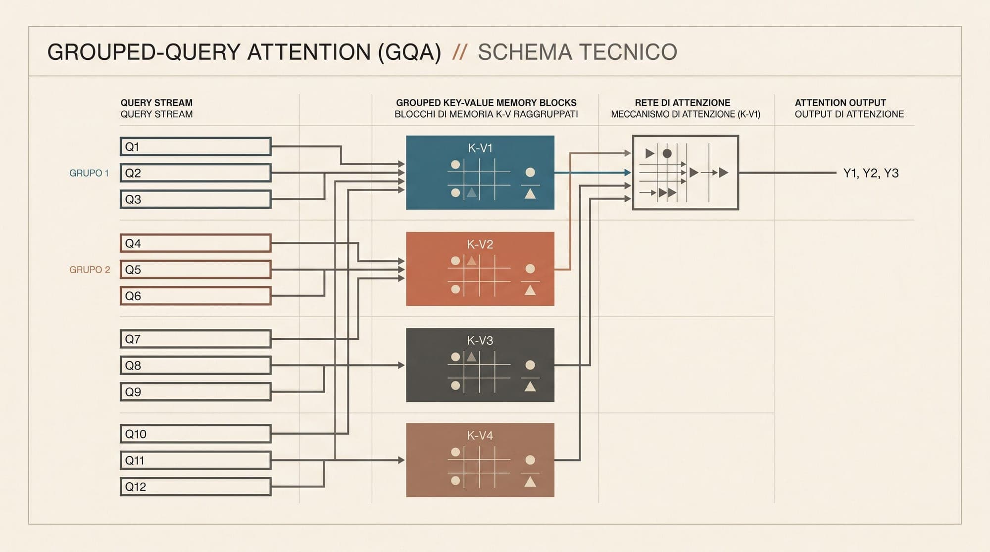
2. Grouped-Query Attention (GQA), introduced by Ainslie et al. (2023), which generalizes MQA by partitioning $H_Q$ query heads into $G$ disjoint groups, with each group sharing a single key-value head pair ($H_K = H_V = G$).

Modern open-weight architectures, including Llama 2 70B and Llama 3, Mistral 7B, and Gemma 2, adopt GQA as the default attention mechanism. This post provides a rigorous breakdown of the memory dynamics, mathematical formulation, hardware roofline mechanics, checkpoint up-training procedures, and serving trade-offs between MHA, MQA, and GQA.

1. The Hardware Bottleneck: Arithmetic Intensity and Memory Bandwidth

To understand why key-value head reduction is essential, consider the operational mechanics of autoregressive decoding on modern GPU hardware such as the NVIDIA H100 SXM5 (3.35 TB/s HBM3 memory bandwidth, 989 TFLOPS dense FP16/BF16 Tensor Core compute).

Arithmetic Intensity in Autoregressive Decoding

The arithmetic intensity $I$ of an operation is defined as the ratio of floating-point operations (FLOPs) performed to bytes transferred from global memory:

$$I = \frac{\text{FLOPs}}{\text{Bytes Transferred}} \quad \left[\frac{\text{FLOP}}{\text{Byte}}\right]$$

According to the roofline model analyzed by Pope et al. (2022), a workload is memory-bandwidth bound if its arithmetic intensity is lower than the hardware operational intensity balance point $I_{\text{sat}} = \frac{\text{Peak FLOPS}}{\text{Peak Memory Bandwidth}}$. For an H100 SXM5 GPU:

$$I_{\text{sat}} = \frac{989 \times 10^{12} \text{ FLOP/s}}{3.35 \times 10^{12} \text{ Byte/s}} \approx 295.2 \text{ FLOP/Byte}$$

During single-batch decoding ($b = 1$) of a single token:

• Loading model weights $W$ requires reading $2 \times P$ bytes (at 16-bit precision), where $P$ is the parameter count.
• Computing the forward pass for a single token requires approximately $2 \times P$ FLOPs.
• The arithmetic intensity of linear projections is $I \approx \frac{2P}{2P} = 1 \text{ FLOP/Byte}$, which is over 200 times lower than $I_{\text{sat}}$.

As a result, the Tensor Cores spend more than 99% of execution cycles stalled waiting for memory transfers from HBM.

KV Cache Memory Footprint

In addition to static model weights, attention requires caching the key and value vectors of all past tokens in the sequence to prevent redundant $O(s^2)$ recomputation. For a model with $L$ layers, hidden dimension $d_{\text{model}}$, sequence length $s$, batch size $b$, and number of key-value heads $H_{KV}$ each with head dimension $d_k = \frac{d_{\text{model}}}{H_Q}$, the total memory required for the KV cache in bytes (using 16-bit floats, 2 bytes per element) is:

$$\text{Memory}_{\text{KV}} = 2 \times 2 \times b \times s \times L \times H_{KV} \times d_k \quad \text{bytes}$$

The leading factor of 2 accounts for storing both Keys and Values, and the second factor of 2 accounts for FP16/BF16 precision.

+-------------------------------------------------------------------------------+
|                      KV CACHE SCALING REGIMES (FP16)                          |
| Model: 70B (L=80, d_model=8192, H_Q=64, d_k=128)                              |
+-------------------+--------------------+------------------+-------------------+
| Sequence Length   | MHA (H_KV = 64)    | GQA-8 (H_KV = 8) | MQA (H_KV = 1)    |
+-------------------+--------------------+------------------+-------------------+
| 4,096 tokens      | 10.74 GB / stream  | 1.34 GB / stream | 0.17 GB / stream  |
| 32,768 tokens     | 85.90 GB / stream  | 10.74 GB / stream| 1.34 GB / stream  |
| 131,072 tokens    | 343.60 GB / stream | 42.95 GB / stream| 5.37 GB / stream  |
+-------------------+--------------------+------------------+-------------------+

Under Multi-Head Attention, a single 128k context stream for a 70B parameter model requires 343.6 GB of VRAM solely for its KV cache, exceeding the total physical memory capacity of four 80GB H100 GPUs. GQA with 8 groups reduces this cache requirement by an exact factor of 8 (42.95 GB), enabling concurrent serving of long-context requests on a single multi-GPU node.

2. Mathematical Formulation: MHA vs. MQA vs. GQA

Let $x \in \mathbb{R}^{b \times s \times d_{\text{model}}}$ denote the input activation tensor, where $b$ is the batch size, $s$ is the sequence length, and $d_{\text{model}}$ is the model hidden dimension. Let $H_Q$ be the number of query heads, and $d_k = d_v = \frac{d_{\text{model}}}{H_Q}$ be the per-head dimension.

Multi-Head Attention (MHA)

In standard Multi-Head Attention, independent linear transformations project the input into $H_Q$ query heads, $H_Q$ key heads, and $H_Q$ value heads:

$$W_Q \in \mathbb{R}^{d_{\text{model}} \times (H_Q \cdot d_k)}, \quad W_K \in \mathbb{R}^{d_{\text{model}} \times (H_Q \cdot d_k)}, \quad W_V \in \mathbb{R}^{d_{\text{model}} \times (H_Q \cdot d_k)}$$

The projections produce:

$$Q = x W_Q \in \mathbb{R}^{b \times s \times H_Q \times d_k}$$ $$K = x W_K \in \mathbb{R}^{b \times s \times H_Q \times d_k}$$ $$V = x W_V \in \mathbb{R}^{b \times s \times H_Q \times d_k}$$

For each head $i \in \{1, \dots, H_Q\}$, the scaled dot-product attention is computed independently:

$$\text{Head}_i = \text{softmax}\left(\frac{Q_i K_i^T}{\sqrt{d_k}} + M\right) V_i$$

where $M \in \mathbb{R}^{s \times s}$ is the causal attention mask. The output projection combines all heads:

$$\text{MHA}(x) = \text{Concat}(\text{Head}_1, \dots, \text{Head}_{H_Q}) W_O, \quad W_O \in \mathbb{R}^{(H_Q \cdot d_k) \times d_{\text{model}}}$$

Multi-Query Attention (MQA)

Multi-Query Attention, proposed by Shazeer (2019), retains $H_Q$ distinct query heads but restricts the key and value projections to a single shared head:

$$W_Q \in \mathbb{R}^{d_{\text{model}} \times (H_Q \cdot d_k)}, \quad W_K \in \mathbb{R}^{d_{\text{model}} \times d_k}, \quad W_V \in \mathbb{R}^{d_{\text{model}} \times d_k}$$

The resulting key and value tensors have no head dimension (or equivalently, a head dimension of 1):

$$Q \in \mathbb{R}^{b \times s \times H_Q \times d_k}, \quad K \in \mathbb{R}^{b \times s \times 1 \times d_k}, \quad V \in \mathbb{R}^{b \times s \times 1 \times d_k}$$

During attention calculation, $K$ and $V$ are broadcast across all $H_Q$ query heads:

$$\text{Head}_i = \text{softmax}\left(\frac{Q_i K^T}{\sqrt{d_k}} + M\right) V$$

While MQA slashes memory bandwidth consumption during decoding by a factor of $H_Q$, it can cause capacity degradation and training instability on complex reasoning and retrieval tasks due to the extreme bottleneck of compressing all token relationships into one key-value subspace.

Grouped-Query Attention (GQA)

Grouped-Query Attention, formulated by Ainslie et al. (2023), interpolates between MHA and MQA. It divides the $H_Q$ query heads into $G$ disjoint groups, where $1 \le G \le H_Q$:

• Group size: $R = \frac{H_Q}{G}$ query heads per group.
• Number of key and value heads: $H_{KV} = G$.
• When $G = H_Q$, GQA reduces exactly to MHA.
• When $G = 1$, GQA reduces exactly to MQA.

The projection weights have shapes:

$$W_Q \in \mathbb{R}^{d_{\text{model}} \times (H_Q \cdot d_k)}, \quad W_K \in \mathbb{R}^{d_{\text{model}} \times (G \cdot d_k)}, \quad W_V \in \mathbb{R}^{d_{\text{model}} \times (G \cdot d_k)}$$

Let $g(i) = \left\lfloor \frac{i-1}{R} \right\rfloor + 1$ denote the group index corresponding to query head $i$. The attention computation for query head $i$ pairs with the shared key and value head of its group $g(i)$:

$$\text{Head}_i = \text{softmax}\left(\frac{Q_i K_{g(i)}^T}{\sqrt{d_k}} + M\right) V_{g(i)}$$

In matrix contraction terms, let $K, V \in \mathbb{R}^{b \times s \times G \times d_k}$. In tensor operations, $K$ and $V$ are expanded to match $Q \in \mathbb{R}^{b \times s \times H_Q \times d_k}$ using a repeat-interleave transformation:

$$\tilde{K} = \text{repeat\_interleave}(K, \text{repeats}=R, \text{dim}=2) \in \mathbb{R}^{b \times s \times H_Q \times d_k}$$ $$\tilde{V} = \text{repeat\_interleave}(V, \text{repeats}=R, \text{dim}=2) \in \mathbb{R}^{b \times s \times H_Q \times d_k}$$

The attention operation is then computed efficiently across all query heads:

$$\text{Attention}(Q, \tilde{K}, \tilde{V}) = \text{softmax}\left(\frac{Q \tilde{K}^T}{\sqrt{d_k}} + M\right) \tilde{V}$$

3. Checkpoint Up-Training: Converting MHA to GQA

Training a large language model from scratch requires millions of GPU hours. A significant contribution of Ainslie et al. (2023) was demonstrating that existing pre-trained MHA checkpoints can be converted to GQA architectures via up-training using only 5% of original pre-training compute.

+-------------------------------------------------------------------------------+
|                       MHA TO GQA CONVERSION PIPELINE                          |
|                                                                               |
|  Pre-trained MHA Weights                                                     |
|  W_K: [d_model, H_Q * d_k] ---> Partition into G groups of R heads            |
|                                                                               |
|  Mean Pooling Projection:                                                     |
|  For group g in {1 ... G}:                                                    |
|      W_K_pooled[g] = (1 / R) * Sum_{h in Group_g} W_K[h]                      |
|      W_V_pooled[g] = (1 / R) * Sum_{h in Group_g} W_V[h]                      |
|                                                                               |
|  Resulting GQA Weights:                                                       |
|  W_K_gqa: [d_model, G * d_k]                                                  |
|  W_V_gqa: [d_model, G * d_k]                                                  |
|                                                                               |
|  Up-Training:                                                                 |
|  Fine-tune converted model on 5% of original pre-training token budget        |
+-------------------------------------------------------------------------------+

Weight Pooling Initialization

To construct the initial GQA projection matrices $W_K^{\text{GQA}} \in \mathbb{R}^{d_{\text{model}} \times (G \cdot d_k)}$ and $W_V^{\text{GQA}} \in \mathbb{R}^{d_{\text{model}} \times (G \cdot d_k)}$ from pre-trained MHA matrices $W_K^{\text{MHA}}$ and $W_V^{\text{MHA}}$:

1. Mean Pooling: The key projection weights belonging to each group $g \in \{1, \dots, G\}$ are averaged:

$$W_K^{\text{GQA}}[g] = \frac{1}{R} \sum_{j=(g-1)R + 1}^{gR} W_K^{\text{MHA}}[j]$$

$$W_V^{\text{GQA}}[g] = \frac{1}{R} \sum_{j=(g-1)R + 1}^{gR} W_V^{\text{MHA}}[j]$$

1. First-Head Selection (Alternative): Selecting only the first head of each group ($W_K^{\text{GQA}}[g] = W_K^{\text{MHA}}[(g-1)R + 1]$). Empirical evaluations show that mean pooling consistently yields lower initial perplexity and faster convergence during up-training compared to single-head selection.

Convergence Dynamics

During up-training on the C4 dataset, Ainslie et al. observed the following convergence patterns:

• Up-trained GQA with $G=8$ (GQA-8) recovered 99.7% of the original MHA model's benchmark performance across downstream tasks (including CNN/DailyMail, MNLI, and SQuAD) within 5% of original pre-training steps.
• Direct MQA conversion ($G=1$) exhibited a larger initial perplexity spike and required longer adaptation to approach MHA performance.
• GQA-8 achieved identical generation throughput to MQA while matching the task accuracy of full MHA.

4. Serving Dynamics and Tensor Parallelism

Deploying GQA models in production inference systems introduces specific constraints and speedups across multi-GPU environments.

Tensor Parallelism (TP) Head Partitioning

In distributed serving frameworks like vLLM and TensorRT-LLM, multi-head attention is partitioned across $N_{\text{TP}}$ GPUs via Megatron-LM tensor parallelism:

• The query projection weight $W_Q$ is split column-wise: each GPU holds $\frac{H_Q}{N_{\text{TP}}}$ query heads.
• The key and value projection weights $W_K, W_V$ are split column-wise: each GPU holds $\frac{H_{KV}}{N_{\text{TP}}}$ key-value heads.
• The output projection weight $W_O$ is split row-wise, followed by an all-reduce collective communication step.

For tensor parallelism to function without head duplication:

$$H_{KV} \pmod{N_{\text{TP}}} = 0$$

For example, Llama 3 70B uses $H_Q = 64$ and $H_{KV} = 8$. It partitions evenly across $N_{\text{TP}} \in \{1, 2, 4, 8\}$ GPUs. On an 8-GPU node ($\text{TP}=8$), each GPU hosts exactly $\frac{64}{8} = 8$ query heads and $\frac{8}{8} = 1$ key-value head, operating locally as an MQA structure without inter-GPU KV cache communication.

If $\text{TP} > H_{KV}$ (for instance, running a model with $H_{KV}=4$ across 8 GPUs), the key-value heads must be broadcast or duplicated across GPUs within each tensor parallel group, increasing redundant memory allocation.

+-------------------------------------------------------------------------------+
|             TENSOR PARALLEL PARTITIONING (Llama 3 70B on TP=8)                |
|                                                                               |
| GPU 0: Q_heads [0..7]   --> KV_head 0 (Local GQA-8 -> MQA behavior)           |
| GPU 1: Q_heads [8..15]  --> KV_head 1                                         |
| GPU 2: Q_heads [16..23] --> KV_head 2                                         |
| GPU 3: Q_heads [24..31] --> KV_head 3                                         |
| GPU 4: Q_heads [32..39] --> KV_head 4                                         |
| GPU 5: Q_heads [40..47] --> KV_head 5                                         |
| GPU 6: Q_heads [48..55] --> KV_head 6                                         |
| GPU 7: Q_heads [56..63] --> KV_head 7                                         |
|                                                                               |
| All-Reduce sum over W_O row-slices yields identical final output.            |
+-------------------------------------------------------------------------------+

Rotary Position Embeddings (RoPE) Interaction

When applying Rotary Position Embeddings (Su et al., 2021), rotational transformations are applied to $Q$ and $K$ representations prior to dot-product evaluation:

$$R_{\Theta, m}^d = \text{diag}\left(R_{\theta_1, m}, R_{\theta_2, m}, \dots, R_{\theta_{d/2}, m}\right)$$

In GQA:

• RoPE is applied to each of the $H_Q$ query heads: $Q_i^{(m)} = R_{\Theta, m} Q_i$.
• RoPE is applied once to each of the $G$ key heads: $K_g^{(m)} = R_{\Theta, m} K_g$.
• The query head $Q_i^{(m)}$ and the transformed group key $K_{g(i)}^{(m)}$ preserve the exact relative positional distance property:

$$\langle Q_i^{(m)}, K_{g(i)}^{(n)} \rangle = \left(Q_i R_{\Theta, m}\right) \left(K_{g(i)} R_{\Theta, n}\right)^T = Q_i R_{\Theta, m-n} K_{g(i)}^T$$

Because RoPE operates per-head on vectors of dimension $d_k$, the mathematical guarantees of relative position encoding remain identical in GQA and MHA.

5. Architectural Comparison and Empirical Trade-offs

The table below summarizes the architectural configurations and serving characteristics across leading open-weight language models.

+--------------------------------------------------------------------------------------------------+
|                            ATTENTION ARCHITECTURES IN PRODUCTION                                 |
+----------------------+--------------------+---------+----------+----------+----------------------+
| Model                | Attention Type     | H_Q     | H_KV     | Group (R)| KV Cache Compression |
+----------------------+--------------------+---------+----------+----------+----------------------+
| Llama 1 (65B)        | MHA                | 64      | 64       | 1        | 1.0x (Baseline)      |
| Llama 2 (70B)        | GQA                | 64      | 8        | 8        | 8.0x reduction       |
| Llama 3 (8B)         | GQA                | 32      | 8        | 4        | 4.0x reduction       |
| Llama 3 (70B)        | GQA                | 64      | 8        | 8        | 8.0x reduction       |
| Mistral 7B           | GQA                | 32      | 8        | 4        | 4.0x reduction       |
| Mixtral 8x7B         | GQA                | 32      | 8        | 4        | 4.0x reduction       |
| Gemma 2 (9B / 27B)   | GQA                | 16 / 32 | 8 / 16   | 2        | 2.0x reduction       |
| Falcon 40B           | MQA                | 64      | 1        | 64       | 64.0x reduction      |
+----------------------+--------------------+---------+----------+----------+----------------------+

Empirical Serving Performance

According to evaluations on NVIDIA A100/H100 clusters running vLLM:

• Serving Throughput: On long-context workloads (32k sequence lengths), GQA-8 achieves up to 4.5x higher token throughput compared to MHA by fitting larger concurrent batch sizes into GPU memory.
• Time-to-First-Token (TTFT): TTFT is largely compute-bound (prefill) and shows minimal variation between MHA and GQA, since total GEMM compute remains comparable.
• Time-Per-Output-Token (TPOT): In memory-bound generation regimes with batch sizes $b \ge 16$, TPOT decreases by 3x to 6x under GQA due to the substantial reduction in HBM bandwidth saturation per decode step.

6. Summary

Grouped-Query Attention resolves the central tension between model quality and serving efficiency in autoregressive Transformers:

• Memory Bandwidth Amortization: Reducing key-value projection heads directly matches the memory-bound constraints of the GPU roofline model during token decoding.
• Tunable Interpolation: Setting $G$ allows system designers to select the optimal operating point between MHA representation capacity ($G=H_Q$) and MQA bandwidth minimization ($G=1$).
• Hardware Alignment: Choosing $G=8$ provides an 8x reduction in KV cache memory footprint with no measurable loss in perplexity or task performance, establishing GQA as the standard attention architecture for modern foundation models.

Sources

• Fast Transformer Decoding: One Write-Head is All You Need (Shazeer, 2019)
• GQA: Training Generalized Multi-Query Transformer Models from Multi-Head Checkpoints (Ainslie et al., 2023)
• Attention Is All You Need (Vaswani et al., 2017)
• Efficiently Scaling Transformer Inference (Pope et al., 2022)
• Llama 2: Open Foundation and Fine-Tuned Chat Models (Touvron et al., 2023)
• Mistral 7B (Jiang et al., 2023)
• Gemma 2: Improving Open Language Models at a Practical Size (Gemma Team, 2024)
• RoFormer: Enhanced Transformer with Rotary Position Embedding (Su et al., 2021)
• vLLM: Efficient Memory Management for Large Language Model Serving with PagedAttention (Kwon et al., 2023)