The Edge of Stability: How Progressive Sharpening and Hessian Dynamics Govern Deep Learning Optimization

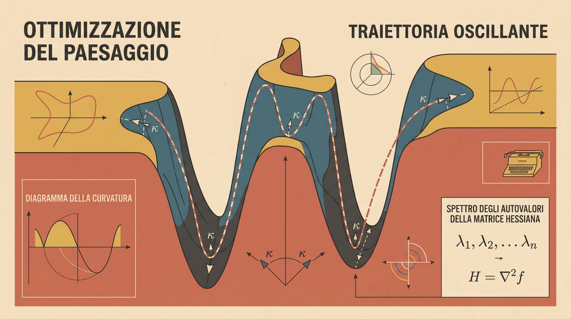
In classical convex optimization, the behavior of gradient descent is dictated by the Lipschitz smoothness constant of the objective function. If a function $f(\theta)$ has an $L$-smooth gradient—meaning the largest eigenvalue of its Hessian matrix is bounded by $\lambda_{\max}(\nabla^2 f(\theta)) \le L$—gradient descent with learning rate $\eta$ is guaranteed to monotonically reduce the loss if and only if $\eta < 2/L$. When the step size exceeds this threshold ($\eta > 2/\lambda_{\max}$), standard quadratic approximations predict catastrophic divergence, with the parameter trajectory oscillating outward toward infinity.

Modern deep neural networks systematically violate this classical stability criterion without diverging. Across architectures spanning convolutional networks, multi-layer perceptrons, and transformers, full-batch and large-batch gradient descent routinely enter a training regime termed the Edge of Stability (EoS). In this regime, the top eigenvalue of the loss Hessian rises to and hovers directly above the theoretical instability threshold $2/\eta$. Instead of blowing up, the network enters a stable limit-cycle or chaotic oscillation along the dominant curvature direction on short timescales, while continuing to make steady optimization progress on long timescales.

Understanding the Edge of Stability resolves long-standing questions regarding why deep networks tolerate large learning rates, how gradient descent navigates non-convex loss surfaces, and why optimization dynamics exhibit an implicit bias toward flatter, generalizable minima.

1. The Classical Paradigm vs. Neural Network Realities

Standard optimization theory relies on the local quadratic approximation of the loss function $L(\theta)$ around the current parameter iterate $\theta_t$:

$$L(\theta_{t+1}) \approx L(\theta_t) + \nabla L(\theta_t)^T (\theta_{t+1} - \theta_t) + \frac{1}{2} (\theta_{t+1} - \theta_t)^T \nabla^2 L(\theta_t) (\theta_{t+1} - \theta_t)$$

Substituting the standard gradient descent update step $\theta_{t+1} = \theta_t - \eta \nabla L(\theta_t)$:

$$L(\theta_{t+1}) \approx L(\theta_t) - \eta \|\nabla L(\theta_t)\|^2 + \frac{\eta^2}{2} \nabla L(\theta_t)^T H(\theta_t) \nabla L(\theta_t)$$

where $H(\theta_t) = \nabla^2 L(\theta_t)$ is the Hessian matrix of second derivatives. Defining local sharpness $S(\theta) = \lambda_{\max}(H(\theta))$ as the largest eigenvalue of the Hessian:

$$L(\theta_{t+1}) - L(\theta_t) \le -\eta \left(1 - \frac{\eta S(\theta_t)}{2}\right) \|\nabla L(\theta_t)\|^2$$

For the loss difference $L(\theta_{t+1}) - L(\theta_t)$ to remain strictly negative (ensuring monotonic descent), the term inside the parentheses must remain positive:

$$1 - \frac{\eta S(\theta_t)}{2} > 0 \implies S(\theta_t) < \frac{2}{\eta}$$

If $S(\theta_t) > 2/\eta$, the quadratic term dominates the linear descent term. In a purely quadratic landscape, iterating along the eigenvector $v_1$ corresponding to $\lambda_{\max}$ leads to exponential divergence:

$$(\theta_{t+1} - \theta^<em>) = (I - \eta H) (\theta_t - \theta^</em>)$$

The projection along $v_1$ evolves as $(1 - \eta \lambda_{\max})^t$, which oscillates with unbounded growth when $|1 - \eta \lambda_{\max}| > 1 \iff \lambda_{\max} > 2/\eta$.

2. Progressive Sharpening and the Transition to EoS

Empirical investigations by Cohen et al. (arXiv:2103.00065) demonstrated that gradient descent on deep neural networks unfolds in distinct phases:

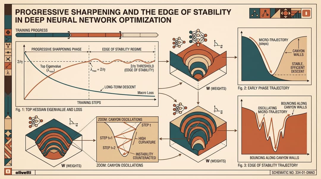
1. Early Phase (Classical Descent): At initialization, network parameters typically sit in flat regions where $\lambda_{\max}(H) \ll 2/\eta$. The loss decreases monotonically, and trajectory dynamics conform closely to continuous-time gradient flow ($\dot{\theta} = -\nabla L(\theta)$).
2. Progressive Sharpening: As parameters move through the optimization landscape and fit training patterns, the local curvature increases. The top eigenvalue $\lambda_{\max}(H)$ climbs steadily across successive iterations.
3. The Edge of Stability Plateau: When $\lambda_{\max}(H)$ reaches the critical threshold $2/\eta$, progressive sharpening ceases. Instead of exceeding $2/\eta$ and triggering explosive divergence, the sharpness saturates and hovers just above $2/\eta$ for the remainder of training.

During the EoS regime, optimization dynamics split across two distinct temporal scales:

• Micro-scale (step-to-step): The training loss behaves non-monotonically, exhibiting high-frequency period-2 or chaotic oscillations. The parameter vector bounces back and forth across the walls of the local quadratic valley along the top eigenvector $v_1$.
• Macro-scale (hundreds of steps): Despite violent local oscillations, the moving average of the training loss continues to descend steadily toward zero.

3. Mathematical Mechanics: Self-Stabilization and Cubic Curvature

Why does the optimizer not diverge when $\lambda_{\max}(H) > 2/\eta$? The explanation lies in higher-order terms of the Taylor series expansion that quadratic approximations discard.

As analyzed by Damian, Nichani, and Lee (arXiv:2209.15594), the third-order directional derivative of the loss function creates a non-linear self-stabilization mechanism. Consider the third-order expansion along the dominant eigenvector $v_1$:

$$L(\theta + \delta v_1) \approx L(\theta) + \delta \nabla L^T v_1 + \frac{1}{2} \delta^2 \lambda_{\max} + \frac{1}{6} \delta^3 \nabla^3 L(v_1, v_1, v_1)$$

When $\lambda_{\max} > 2/\eta$, an update step along $v_1$ overshoots the minimum of the quadratic approximation. In asymmetric or non-quadratic valleys, the local Hessian is state-dependent:

$$\nabla^2 L(\theta + \delta v_1) \approx H(\theta) + \delta \nabla^3 L(v_1, v_1, \cdot)$$

When gradient descent overshoots and lands on a region with asymmetric cubic curvature, the resulting gradient update does not merely reverse direction along $v_1$; it induces a transverse displacement perpendicular to $v_1$. This lateral displacement shifts the parameter trajectory into neighboring regions of the parameter space where the local curvature $\lambda_{\max}(H)$ is lower.

This interaction produces a dynamical feedback loop:

1. If $\lambda_{\max}$ rises above $2/\eta$, gradient descent steps become unstable along $v_1$, amplifying oscillation amplitude.
2. Larger oscillations explore outer regions of the valley, activating cubic and quartic terms that push the parameters laterally into flatter sub-basins.
3. Entering flatter regions reduces $\lambda_{\max}$ back toward $2/\eta$.
4. If $\lambda_{\max}$ falls below $2/\eta$, progressive sharpening resumes until $\lambda_{\max} \approx 2/\eta$ is restored.

The system dynamically regulates its own curvature, locking the trajectory onto the manifold where $\lambda_{\max}(H) \approx 2/\eta$.

4. Implicit Bias Toward Flat Minima

The discovery of the Edge of Stability provides a mechanistic explanation for why training with larger learning rates often yields better generalization performance on unseen test data, a phenomenon noted by Keskar et al. (arXiv:1609.04836) and Dinh et al. (arXiv:1703.04933).

In an optimization landscape containing multiple local minima of varying sharpness:

• Small Learning Rates ($\eta \to 0$): Gradient descent tracks continuous gradient flow. It can enter and settle into narrow, sharp ravines where $\lambda_{\max}(H)$ is high, because the stability condition $\lambda_{\max} < 2/\eta$ is never violated.
• Large Learning Rates (EoS Regime): Any basin where the local minimum has sharpness $S > 2/\eta$ is dynamically unstable. Gradient descent cannot converge to a sharp minimum; the destabilizing oscillations along $v_1$ eject the trajectory from sharp valleys, forcing the optimizer to continue searching until it finds a broad, flat basin where $S \le 2/\eta$.

EoS acts as an implicit regularizer that automatically prunes sharp minima from the set of reachable solutions, selecting flat minima with lower generalization error.

5. Extensions: Momentum, Adaptive Optimizers, and Non-Euclidean Metrics

While initial formulations focused on vanilla full-batch gradient descent, subsequent research has mapped the Edge of Stability across practical deep learning optimizers:

Momentum Methods

For Polyak momentum (heavy-ball) with momentum parameter $\beta \in [0, 1)$, classical linear stability analysis places the stability threshold at:

$$\lambda_{\max}(H) \le \frac{2(1 + \beta)}{\eta}$$

Under Nesterov accelerated gradient descent, the effective threshold shifts to:

$$\lambda_{\max}(H) \le \frac{2(1 + \beta)}{\eta (1 + 2\beta)}$$

Empirical studies confirm that momentum optimizers enter an identical EoS regime, with sharpness hovering around their respective modified stability boundaries.

Adaptive Optimizers (Adam and RMSProp)

In adaptive gradient algorithms, the effective metric is non-Euclidean. The update step is preconditioned by a diagonal matrix $D_t \approx \text{diag}(\sqrt{v_t} + \epsilon)^{-1}$.

The relevant curvature metric is no longer the raw Hessian eigenvalue $\lambda_{\max}(H)$, but the maximum generalized eigenvalue of the preconditioned Hessian:

$$S_{\text{adaptive}}(\theta) = \lambda_{\max}(D_t H(\theta))$$

As shown in recent non-Euclidean optimization frameworks (such as Mishkin et al., arXiv:2405.05313), adaptive optimizers exhibit directional progressive sharpening in the preconditioned metric space, operating at the boundary $S_{\text{adaptive}} \approx 2/\eta$.

6. Practical Implications for Large-Scale Model Training

The Edge of Stability directly impacts the stability and efficiency of large language model (LLM) pre-training:

1. Learning Rate Warmup: At initialization, models undergo rapid structural adaptation. Without learning rate warmup, large initial steps can push the optimizer into extreme instability before self-stabilization dynamics establish. Warmup allows controlled progressive sharpening to reach the EoS boundary gradually.
2. Multi-Frequency Instabilities and Loss Spikes: While self-stabilization easily manages instability along a single dominant eigenvector $v_1$, pre-training large models occasionally produces scenarios where multiple orthogonal directions simultaneously exceed $2/\eta$. When higher-order interactions cross-couple across multiple unstable directions, the self-stabilizing restoring force can break down, manifesting as sudden loss spikes observed during LLM runs.
3. Curvature Diagnostics: Monitoring the Hessian spectral norm $\lambda_{\max}(H)$ via power iteration or the Lanczos algorithm provides a direct operational health metric. Tracking the ratio $\eta \cdot \lambda_{\max}(H) / 2$ reveals whether training is operating safely in the EoS regime ($\approx 1.0$) or approaching catastrophic multi-axis instability ($> 1.5$).

Sources

• Cohen, J. M., Kaur, S., Li, Y., Kolter, J. Z., & Talwalkar, A. (2021). Gradient Descent on Neural Networks Typically Operates at the Edge of Stability. International Conference on Learning Representations (ICLR). arXiv:2103.00065
• Damian, A., Nichani, E., & Lee, J. D. (2023). Self-Stabilization: The Implicit Bias of Gradient Descent at the Edge of Stability. International Conference on Learning Representations (ICLR). arXiv:2209.15594
• Keskar, N. S., Mudigere, D., Nocedal, J., Smelyanskiy, M., & Tang, P. T. P. (2016). On Large-Batch Training for Deep Learning: Generalization Gap and Sharp Minima. International Conference on Learning Representations (ICLR). arXiv:1609.04836
• Dinh, L., Pascanu, R., Bengio, S., & Bengio, Y. (2017). Sharp Minima Can Generalize For Deep Nets. International Conference on Machine Learning (ICML). arXiv:1703.04933
• Mishkin, A., et al. (2024). Directional Smoothness and the Edge of Stability in Deep Learning. International Conference on Machine Learning (ICML). arXiv:2405.05313
• Hochreiter, S., & Schmidhuber, J. (1997). Flat Minima. Neural Computation, 9(1), 1-42. DOI:10.1162/neco.1997.9.1.1