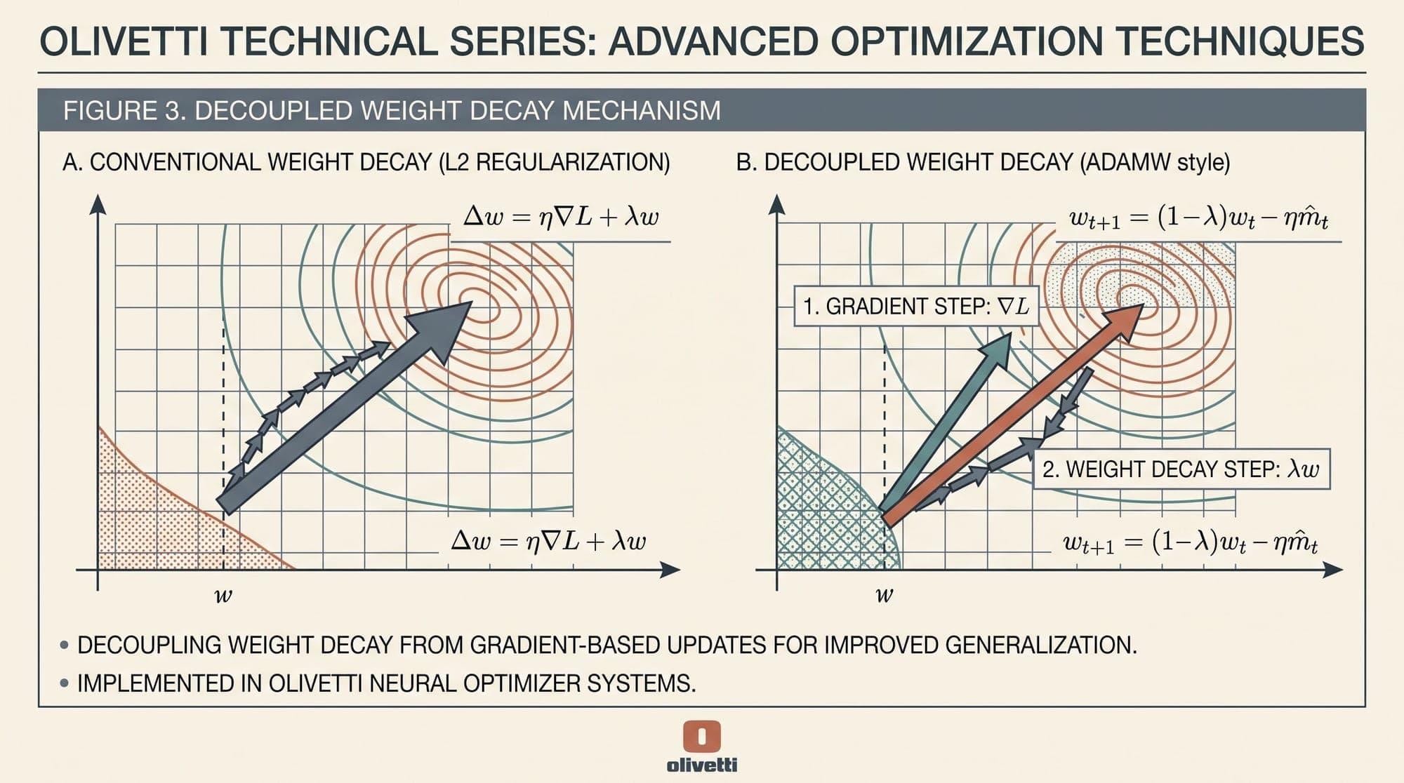
Decoupled Weight Decay Regularization (AdamW): Mathematical Foundations, L2 Regularization Failure in Adaptive Gradient Methods, and Hyperparameter Dynamics

Decoupled weight decay regularization, formalized by Ilya Loshchilov and Frank Hutter in 2017 and published at ICLR 2019, resolved a fundamental flaw in how adaptive gradient algorithms like Adam implemented weight regularization. Prior to AdamW, deep learning frameworks implemented weight decay as L2 regularization by adding the gradient of the squared L2 norm directly to the loss gradient. While mathematically identical for standard stochastic gradient descent (SGD), this formulation breaks down in adaptive optimizers, causing parameters with large or frequent gradients to receive negligible regularization and parameters with sparse gradients to be excessively penalized.

Today, AdamW serves as the standard optimization algorithm across large language model architectures, including LLaMA, GPT, Mistral, and Claude. Understanding its mathematical mechanics reveals why decoupled weight decay is essential for stabilizing deep neural network training.

The Classical Equivalence in SGD

In standard stochastic gradient descent, optimization minimizes an empirical loss function $f(\theta)$ parameterized by weights $\theta \in \mathbb{R}^d$. Regularization can be introduced through two distinct mechanisms: objective modification via L2 penalty or update rule modification via weight decay.

In L2 regularization, the loss function is augmented with a penalty term proportional to the squared Euclidean norm of the parameters:

$$\mathcal{L}_{\text{L2}}(\theta) = f(\theta) + \frac{\lambda}{2} \|\theta\|_2^2$$

Computing the gradient with respect to $\theta$ yields:

$$\nabla \mathcal{L}_{\text{L2}}(\theta) = \nabla f(\theta) + \lambda \theta$$

Applying a standard gradient step with learning rate $\eta_t$ produces the parameter update:

$$\theta_{t+1} = \theta_t - \eta_t \nabla \mathcal{L}_{\text{L2}}(\theta_t) = \theta_t - \eta_t (\nabla f(\theta_t) + \lambda \theta_t) = (1 - \eta_t \lambda)\theta_t - \eta_t \nabla f(\theta_t)$$

In weight decay, first formulated by Hanson and Pratt (1988), the parameters are exponentially shrunk at each step by a decay factor $\lambda'$ prior to performing the loss gradient update:

$$\theta_{t+1} = (1 - \lambda')\theta_t - \eta_t \nabla f(\theta_t)$$

Comparing the two update equations shows that setting $\lambda' = \eta_t \lambda$ makes L2 regularization and weight decay algebraically identical in standard SGD. Because of this identity, early deep learning libraries used the terms interchangeably and implemented weight decay simply by adding $\lambda \theta$ to the computed gradient $\nabla f(\theta)$.

The Breakdown in Adaptive Gradient Methods

Adaptive gradient algorithms adjust effective step sizes on a per-coordinate basis using historical gradient statistics. Adam maintains exponentially moving averages of past gradients ($m_t$) and past squared gradients ($v_t$):

$$m_t = \beta_1 m_{t-1} + (1 - \beta_1) g_t$$

$$v_t = \beta_2 v_{t-1} + (1 - \beta_2) g_t^2$$

$$\hat{m}_t = \frac{m_t}{1 - \beta_1^t}, \quad \hat{v}_t = \frac{v_t}{1 - \beta_2^t}$$

When L2 regularization is applied, the combined gradient $g_t = \nabla f_t(\theta_t) + \lambda \theta_t$ enters both the first moment $m_t$ and the second moment $v_t$. The parameter update becomes:

$$\theta_{t+1} = \theta_t - \eta_t \frac{\hat{m}_t}{\sqrt{\hat{v}_t} + \epsilon}$$

Expanding the update for a simplified scenario where momentum is negligible reveals the core issue:

$$\theta_{t+1} \approx \theta_t - \eta_t \frac{\nabla f_t(\theta_t) + \lambda \theta_t}{\sqrt{v_t} + \epsilon} = \theta_t - \eta_t \frac{\lambda \theta_t}{\sqrt{v_t} + \epsilon} - \eta_t \frac{\nabla f_t(\theta_t)}{\sqrt{v_t} + \epsilon}$$

The effective weight decay rate applied to parameter $\theta_{i,t}$ is:

$$\lambda_{\text{eff}, i} = \frac{\eta_t \lambda}{\sqrt{v_{i,t}} + \epsilon}$$

This introduces two severe structural failure modes:

1. Inverse Variance Scaling: For parameters that receive large and frequent gradients, $v_{i,t}$ is large, causing $\lambda_{\text{eff}, i} \to 0$. These parameters receive almost zero weight shrinkage, preventing effective regularization where capacity control is most critical.
2. Sparse Gradient Amplification: For parameters that receive small or infrequent gradients (such as rare embedding tokens), $v_{i,t}$ is small, causing $\lambda_{\text{eff}, i} \to \frac{\eta_t \lambda}{\epsilon}$. These weights are aggressively penalized, distorting learned representations.

Furthermore, because $\lambda \theta_t$ enters $v_t$, a large weight norm artificially inflates $v_t$, which in turn reduces the effective learning rate for the loss gradient $\nabla f_t(\theta_t)$.

Mathematical Derivation of AdamW

Loshchilov and Hutter proposed decoupling the regularization step from the adaptive gradient moment updates. In AdamW, the gradient statistics track only the loss gradient $\nabla f_t(\theta_t)$, and parameter decay is subtracted directly from $\theta_t$:

$$g_t = \nabla f_t(\theta_t)$$

$$m_t = \beta_1 m_{t-1} + (1 - \beta_1) g_t$$

$$v_t = \beta_2 v_{t-1} + (1 - \beta_2) g_t^2$$

$$\hat{m}_t = \frac{m_t}{1 - \beta_1^t}, \quad \hat{v}_t = \frac{v_t}{1 - \beta_2^t}$$

$$\theta_{t+1} = (1 - \eta_t \lambda) \theta_t - \eta_t \frac{\hat{m}_t}{\sqrt{\hat{v}_t} + \epsilon}$$

In the normalized formulation proposed in the original paper, weight decay is scaled by the scheduled learning rate relative to the initial learning rate $\eta_0$:

$$\theta_{t+1} = \theta_t - \eta_t \frac{\hat{m}_t}{\sqrt{\hat{v}_t} + \epsilon} - \eta_t \lambda \theta_t$$

By subtracting $\eta_t \lambda \theta_t$ outside the adaptive fraction:

• Every parameter decays at an identical relative rate proportional to its current magnitude, independent of historical gradient variance.
• Gradient second moments $v_t$ reflect purely the variance and curvature of the objective function $f(\theta)$.
• The gradient step direction is unaffected by the magnitude of the weight vector.

Hyperparameter Disentanglement and Scheduling

A major operational benefit of AdamW is the separation of optimal learning rate $\eta$ and optimal weight decay coefficient $\lambda$.

Under standard Adam with L2 regularization, changing the learning rate schedule (for example, switching from step decay to cosine annealing) alters the effective regularization rate throughout training. If $\eta_t$ drops by two orders of magnitude, the effective L2 penalty also drops proportionally, coupling the grid search space of $\eta$ and $\lambda$.

In AdamW:

• When learning rate $\eta$ is tuned, the optimal weight decay $\lambda$ remains largely constant.
• With cosine learning rate schedules, decaying both the step size $\eta_t$ and the weight shrinkage rate proportionally ensures that late-stage fine-tuning avoids destroying stabilized feature representations while maintaining equilibrium at flat minima.

Empirical Impact on Transformer Scaling

In large language model pre-training, AdamW provides critical stability advantages over standard Adam:

1. Embedding and Head Stability: Output projection heads and token embedding matrices experience highly non-uniform token frequencies. Under L2 regularization, rare token embeddings are shrunk excessively while frequent token vectors grow unbounded. AdamW maintains uniform norm bounds across vocabulary dimensions.
2. Attention Logit Drift: In deep transformer blocks, unregularized weights in query-key projections lead to large activation norms, causing attention logits to grow and attention distributions to saturate into one-hot distributions. AdamW prevents weight norm explosion across deep layers without dampening active gradient flow.
3. Generalization at the Edge of Stability: Empirical studies on neural scaling demonstrate that AdamW consistently achieves lower validation perplexity and improved downstream zero-shot accuracy compared to Adam with L2 regularization across matched compute budgets.

Practical Implementation

In modern frameworks such as PyTorch, torch.optim.AdamW implements decoupled weight decay directly. The core update loop executes:

# PyTorch AdamW step execution logic
for p in parameters:
    if p.grad is None:
        continue
    grad = p.grad
    state = optimizer.state[p]

    # State initialization
    if len(state) == 0:
        state['step'] = 0
        state['exp_avg'] = torch.zeros_like(p)
        state['exp_avg_sq'] = torch.zeros_like(p)

    exp_avg, exp_avg_sq = state['exp_avg'], state['exp_avg_sq']
    state['step'] += 1

    # Perform step-level weight decay
    if weight_decay != 0:
        p.data.mul_(1.0 - lr * weight_decay)

    # Decay the first and second moment running average coefficient
    exp_avg.mul_(beta1).add_(grad, alpha=1 - beta1)
    exp_avg_sq.mul_(beta2).addcmul_(grad, grad, value=1 - beta2)

    denom = (exp_avg_sq.sqrt() / math.sqrt(bias_correction2)).add_(eps)
    step_size = lr / bias_correction1

    p.data.addcdiv_(exp_avg, denom, value=-step_size)

By applying p.data.mul_(1.0 - lr * weight_decay) directly to the parameter buffer before computing the moment-based update, PyTorch ensures exact adherence to the decoupled formulation.

Sources

• Decoupled Weight Decay Regularization (Loshchilov & Hutter, 2017/2019)
• Adam: A Method for Stochastic Optimization (Kingma & Ba, 2014)
• Comparing Biases for Minimal Network Construction with Back-Propagation (Hanson & Pratt, 1988)
• Understanding Decoupled and Early Weight Decay (Bjorck et al., AAAI 2021)
• PyTorch AdamW Implementation Reference