Layer Normalization and RMSNorm in Large Language Models: How Pre-LN, Scaling Invariance, and QK-Norm Stabilize Deep Transformers

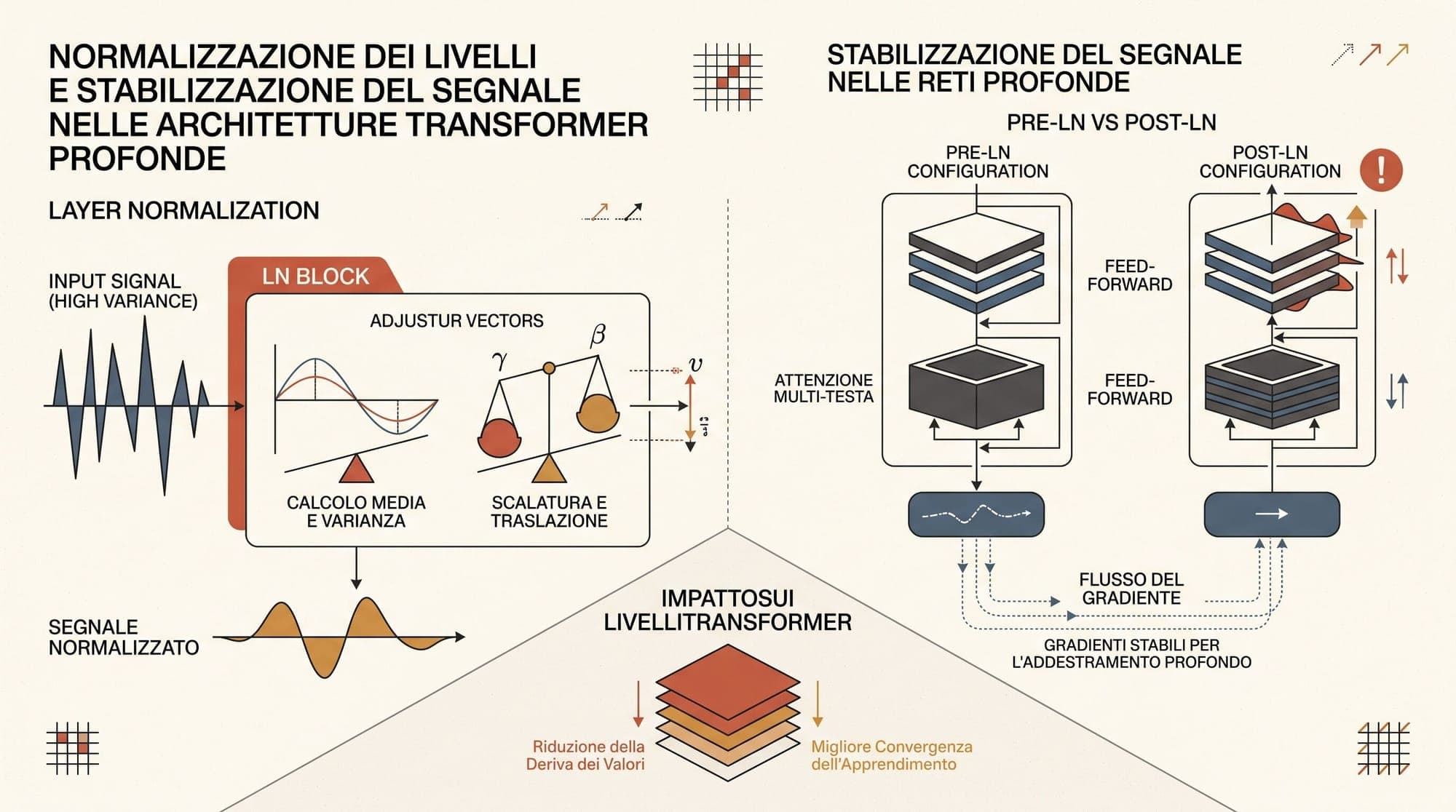
Training deep autoregressive Transformers requires maintaining numerical stability across dozens or hundreds of stacked attention and feed-forward blocks. As models scale from 7 billion to hundreds of billions of parameters, uncontrolled variance growth along the residual stream or unbounded attention logits can trigger catastrophic loss spikes, gradient underflow, or numerical divergence.

Normalization layers act as the primary stabilizing mechanism in modern Large Language Models (LLMs). While the original Transformer architecture relied on standard Layer Normalization (LayerNorm) placed after residual connections, contemporary frontier models (including Meta's LLaMA series, Mistral, Google's Gemma, Qwen, and DeepSeek) have converged on a refined architectural stack: Pre-LayerNorm placement, Root Mean Square Layer Normalization (RMSNorm), and Query-Key Normalization (QK-Norm).

This explainer examines the mathematical mechanics, architectural trade-offs, and hardware execution realities of normalization layers in modern LLMs.

The Normalization Bottleneck in Deep Transformers

In deep neural networks, activations passing through unconstrained linear transformations and non-linearities experience internal covariate shift and cumulative variance expansion. Without normalization, intermediate representations either explode exponentially with depth or collapse toward zero, driving gradients outside representable floating-point ranges.

In computer vision and convolutional architectures, Batch Normalization (Ioffe & Szegedy, 2015) addresses this by computing mean and variance across mini-batch samples for each channel. However, Batch Normalization breaks down in autoregressive language models due to three fundamental issues:

1. Variable Sequence Lengths: Natural language tokens vary dynamically across batches, requiring complex padding masks that distort batch-level statistics.
2. Autoregressive Inference Dependencies: During single-token generation at inference time (batch size 1), mini-batch statistics are unavailable, requiring static running averages that often drift from dynamic conversational contexts.
3. Distributed Communication Overhead: In distributed training frameworks utilizing Tensor Parallelism or Pipeline Parallelism, calculating batch-level statistics introduces cross-device synchronization latency across GPU clusters.

To resolve these constraints, Layer Normalization (Ba, Kiros, & Hinton, 2016) shifts the statistical reduction from the batch dimension to the feature (hidden) dimension. Each token vector is normalized independently across its hidden channels, making the operation invariant to batch size and sequence length.

Architectural Placement: Post-LN, Pre-LN, and DeepNorm

The positioning of normalization relative to the multi-head attention and feed-forward sublayers profoundly alters gradient dynamics during backpropagation.

1. Post-LayerNorm (Post-LN)

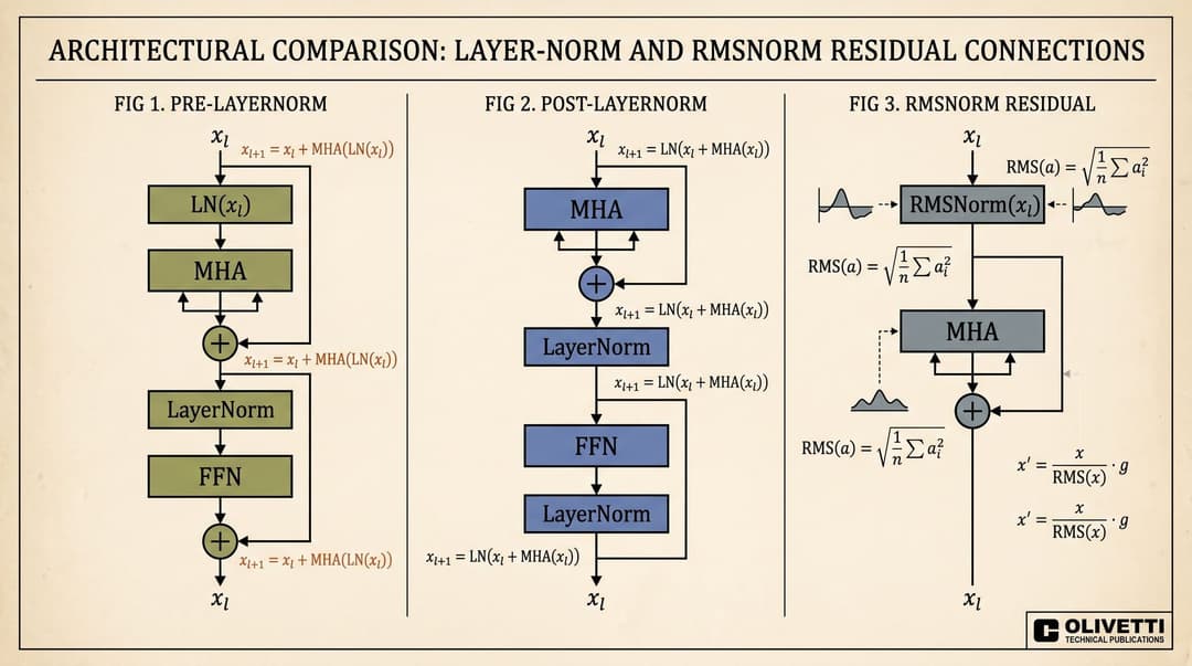
In the original Transformer architecture (Vaswani et al., 2017), normalization is applied after the residual addition:

$$x_{l+1} = \text{LayerNorm}(x_l + \text{SubLayer}(x_l))$$

While Post-LN provides strong representation capacity by preventing the unnormalized residual stream from growing, it introduces severe optimization challenges. As proven by Xiong et al. (2020), the expected gradient norm near the output layer is significantly larger than near the input layers. Gradients propagating backward through consecutive LayerNorm operations decay at a rate proportional to $O(1/\sqrt{L})$, where $L$ is total model depth.

As a result, training deep Post-LN Transformers without a careful learning rate warmup phase causes early gradient instability and training divergence.

2. Pre-LayerNorm (Pre-LN)

To eliminate the strict dependency on delicate warmup schedules, modern LLMs adopt Pre-LayerNorm placement (Radford et al., 2019; Xiong et al., 2020):

$$x_{l+1} = x_l + \text{SubLayer}(\text{LayerNorm}(x_l))$$

In Pre-LN, the residual connection functions as an uninterrupted identity highway ($x_L = x_0 + \sum_{l=0}^{L-1} \text{SubLayer}(\text{LayerNorm}(x_l))$). Gradients flow directly from the loss function to early layers without passing through intermediate normalization derivatives. This allows models to train stably from step zero at higher learning rates.

However, Pre-LN introduces a subtle side effect: the magnitude (norm) of the residual stream vector $x_l$ grows with depth as $O(\sqrt{L})$. Because the inputs to deeper layers have increasingly large norms while the sublayer output magnitudes remain bounded by normalization, each successive layer contributes a smaller relative percentage change to the residual stream. This phenomenon, termed representation collapse or depth attenuation, means that very deep Pre-LN layers can behave similarly to identity mappings.

3. DeepNorm

To reconcile the stability of Pre-LN with the high capacity of Post-LN, Microsoft Research introduced DeepNorm (DeepNet) (Wang et al., 2022). DeepNorm modifies the residual addition with a constant scaling factor $\beta$ while scaling the initialization of parameter weights inside the sublayer by $\alpha$:

$$x_{l+1} = \text{LayerNorm}(x_l \cdot \beta + \text{SubLayer}(x_l))$$

$$\beta = (2N)^{-\frac{1}{4}}, \quad \alpha = (2N)^{-\frac{1}{4}} \quad (\text{for encoder-decoder architectures})$$

By bounding the expected update variance at each residual junction to a constant upper bound, DeepNorm enables stable training of Transformers scaling past 1,000 layers without divergence.

Mathematical Formulation: LayerNorm vs. RMSNorm

Standard Layer Normalization centers activations around a zero mean and scales them to unit variance, followed by a learned affine transformation.

Standard LayerNorm Formulation

Given a token hidden vector $x \in \mathbb{R}^d$:

1. Compute the mean across the hidden dimension:

$$\mu = \frac{1}{d} \sum_{i=1}^d x_i$$

1. Compute the variance:

$$\sigma^2 = \frac{1}{d} \sum_{i=1}^d (x_i - \mu)^2$$

1. Normalize and apply learned gain $\gamma \in \mathbb{R}^d$ and bias $\beta \in \mathbb{R}^d$:

$$\bar{x}_i = \frac{x_i - \mu}{\sqrt{\sigma^2 + \epsilon}} \cdot \gamma_i + \beta_i$$

Where $\epsilon > 0$ is a small constant (e.g., $10^{-5}$ or $10^{-6}$) to prevent division by zero.

Root Mean Square Layer Normalization (RMSNorm)

In 2019, Zhang & Sennrich investigated the underlying mechanism behind LayerNorm's regularization success. They hypothesized that the computational overhead of re-centering invariance (subtracting $\mu$) is dispensable, and that the regularizing power of LayerNorm stems entirely from re-scaling invariance (dividing by the root mean square magnitude).

RMSNorm modifies the formulation by dropping the mean calculation and the learned shift parameter $\beta$:

1. Compute the root mean square statistic:

$$\text{RMS}(x) = \sqrt{\frac{1}{d} \sum_{i=1}^d x_i^2 + \epsilon}$$

1. Scale the input vector by the root mean square and apply the learned gain $\gamma$:

$$\bar{x}_i = \frac{x_i}{\text{RMS}(x)} \cdot \gamma_i$$

import torch
import torch.nn as nn

class RMSNorm(nn.Module):
    """
    Root Mean Square Layer Normalization (Zhang & Sennrich, 2019).
    Dropping mean calculation and bias saves memory bandwidth and kernel latency.
    """
    def __init__(self, dim: int, eps: float = 1e-6):
        super().__init__()
        self.eps = eps
        self.weight = nn.Parameter(torch.ones(dim))

    def forward(self, x: torch.Tensor) -> torch.Tensor:
        # x shape: [batch_size, seq_len, dim]
        variance = x.pow(2).mean(dim=-1, keepdim=True)
        x_normed = x * torch.rsqrt(variance + self.eps)
        return self.weight * x_normed

Computational and Memory Benefits

Eliminating the mean subtraction provides substantial systems-level advantages:

• Reduced Memory Passes: In a standard LayerNorm forward pass, the GPU must compute the mean across $d$ dimensions, perform a second reduction to compute variance relative to that mean, and then execute an element-wise subtraction and scaling. RMSNorm requires only a single reduction pass ($x_i^2$).
• Fewer Parameters: Dropping the learnable bias vector $\beta$ reduces parameter storage and optimizer state memory in AdamW (which tracks first and second gradient moments for each parameter).
• Latency Speedup: On modern accelerator hardware, normalization is strictly memory-bandwidth bound. RMSNorm reduces kernel execution time by 7% to 50% compared to standard LayerNorm depending on the hidden dimension and GPU memory hierarchy, with identical convergence rates across billions of pre-training tokens.

Frontier Numerical Stability: Gemma Offset, QK-Norm, and Logit Capping

As open-weight models have grown in scale and shifted toward low-precision FP8 and BF16 mixed-precision pre-training, modern architectures implement several targeted extensions to baseline RMSNorm.

1. Gemma Unit Offset RMSNorm

In Google's Gemma and Gemma 2 architectures, standard RMSNorm scaling is modified with a unit offset:

$$\bar{x}_i = \frac{x_i}{\text{RMS}(x)} \cdot (1 + w_i)$$

The weight parameter $w_i$ is initialized to zero rather than one. This ensures that at step zero, the layer represents an exact mathematical identity without risking numerical drift during weight initialization or optimizer state updates.

2. Query-Key Normalization (QK-Norm)

In standard Multi-Head Attention, attention logits are computed as:

$$\text{Attention}(Q, K, V) = \text{softmax}\left(\frac{Q K^T}{\sqrt{d_k}}\right) V$$

As Transformer models scale to tens of billions of parameters, the magnitudes of unnormalized query ($Q$) and key ($K$) vector projections can drift upward over millions of training steps. When the dot product $Q K^T$ grows significantly larger than $\sqrt{d_k}$, attention logits reach extreme values ($> 100$).

When passed into the softmax function, large logits cause severe softmax saturation: one attention score approaches 1.0 while all others collapse to 0.0. This destroys attention entropy, causes vanishing gradients across attention heads, and triggers catastrophic loss spikes or NaN values in FP16/BF16 arithmetic.

To eliminate this vulnerability, Dehghani et al. (2023) in ViT-22B and Wortsman et al. (2023) introduced Query-Key Normalization (QK-Norm). QK-Norm applies an RMSNorm or LayerNorm operation directly to the Query and Key vectors after their linear projections but prior to the rotary embedding application and dot product:

$$Q_{\text{norm}} = \text{RMSNorm}(Q), \quad K_{\text{norm}} = \text{RMSNorm}(K)$$

$$\text{Attention}(Q, K, V) = \text{softmax}\left(\frac{Q_{\text{norm}} K_{\text{norm}}^T}{\sqrt{d_k}}\right) V$$

Because the $L_2$ norm of each head vector is strictly constrained, attention logits cannot expand unboundedly. QK-Norm has become standard across frontier architectures, including Alibaba's Qwen 2.5/3 series, Google's Gemma 2, and Cohere's Command R+.

class NormalizedAttention(nn.Module):
    """
    Multi-Head Attention with QK-Norm to prevent attention logit explosion.
    """
    def __init__(self, dim: int, num_heads: int, head_dim: int):
        super().__init__()
        self.num_heads = num_heads
        self.head_dim = head_dim
        self.scale = head_dim ** -0.5

        self.q_proj = nn.Linear(dim, num_heads * head_dim, bias=False)
        self.k_proj = nn.Linear(dim, num_heads * head_dim, bias=False)
        self.v_proj = nn.Linear(dim, num_heads * head_dim, bias=False)
        self.o_proj = nn.Linear(num_heads * head_dim, dim, bias=False)

        # Per-head RMSNorm for Q and K
        self.q_norm = RMSNorm(head_dim)
        self.k_norm = RMSNorm(head_dim)

    def forward(self, x: torch.Tensor, mask: torch.Tensor = None) -> torch.Tensor:
        b, s, _ = x.shape
        q = self.q_proj(x).view(b, s, self.num_heads, self.head_dim)
        k = self.k_proj(x).view(b, s, self.num_heads, self.head_dim)
        v = self.v_proj(x).view(b, s, self.num_heads, self.head_dim)

        # Apply QK-Norm prior to dot product
        q = self.q_norm(q).transpose(1, 2)  # [b, num_heads, s, head_dim]
        k = self.k_norm(k).transpose(1, 2)
        v = v.transpose(1, 2)

        # Bounded attention logits
        scores = torch.matmul(q, k.transpose(-2, -1)) * self.scale
        if mask is not None:
            scores = scores + mask
            
        attn = torch.softmax(scores, dim=-1)
        out = torch.matmul(attn, v).transpose(1, 2).contiguous().view(b, s, -1)
        return self.o_proj(out)

3. Attention Logit Soft-Capping

Complementing QK-Norm, architectures such as Gemma 2 and xAI's Grok implement soft-capping on attention logits:

$$\text{logits}_{\text{capped}} = \text{cap} \cdot \tanh\left(\frac{Q K^T}{\text{cap} \cdot \sqrt{d_k}}\right)$$

Where $\text{cap}$ is set to a constant threshold (such as 50.0 for attention logits and 30.0 for final vocabulary projection logits). Even if numerical anomalies occur in query-key projections, the hyperbolic tangent function clamps logit outputs strictly into the range $[-\text{cap}, \text{cap}]$, guaranteeing stable softmax evaluation across multi-trillion-token training runs.

Hardware Execution: Kernel Fusion and SRAM Memory Traffic

From a hardware execution standpoint, normalization layers have an arithmetic intensity of less than 1 FLOP per byte transferred from GPU High Bandwidth Memory (HBM). Without operator fusion, calculating RMSNorm requires writing intermediate activations to HBM, reloading them for the root-mean-square calculation, and writing the normalized results back out.

To eliminate this memory bandwidth bottleneck, modern inference and training runtimes (such as FlashAttention, vLLM, SGLang, and Triton) implement Fused RMSNorm Kernels:

1. Warp-Level Reductions: Threads within a CUDA warp (32 threads) perform parallel tree reductions using warp shuffle intrinsics (__shfl_xor_sync / __shfl_down_sync), computing the sum-of-squares across the hidden dimension entirely inside GPU registers without touching shared memory or HBM.
2. Fused Residual Connections: In Pre-LN Transformers, the addition of the residual stream ($x_{l+1} = x_l + \text{output}_l$) and the subsequent layer's RMSNorm ($\text{RMSNorm}(x_{l+1})$) are fused into a single GPU kernel call. The unnormalized sum is written to HBM for future residual addition while the normalized output is retained in SRAM/registers for immediate input into the next projection matrix.

By combining Pre-LN residual connections, fused RMSNorm kernels, and Query-Key normalization, modern LLM architectures achieve high training throughput while maintaining continuous numerical stability across massive pre-training runs.

Sources

• Ba, J. L., Kiros, J. R., & Hinton, G. E. (2016). Layer Normalization. arXiv:1607.06450
• Zhang, B., & Sennrich, R. (2019). Root Mean Square Layer Normalization. NeurIPS 2019. arXiv:1910.07467
• Vaswani, A., et al. (2017). Attention Is All You Need. NeurIPS 2017. arXiv:1706.03762
• Xiong, R., et al. (2020). On Layer Normalization in the Transformer Architecture. ICML 2020. arXiv:2002.04745
• Wang, H., et al. (2022). DeepNet: Scaling Transformers to 1,000 Layers. arXiv:2203.00555
• Dehghani, M., et al. (2023). Scaling Vision Transformers to 22 Billion Parameters. arXiv:2302.05442
• Wortsman, M., et al. (2023). Small-scale proxies for large-scale Transformer training stability. arXiv:2309.14322
• Gemma Team, Google. (2024). Gemma: Open Models Based on Gemini Research and Technology. arXiv:2403.08295