Grokking in Large Language Models: How Weight Decay and Circuit Efficiency Drive Delayed Generalization

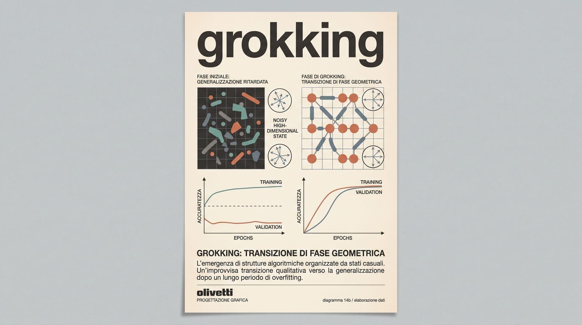
In standard machine learning paradigms, model generalization closely tracks training loss: as an optimizer minimizes loss on training data, performance on held-out validation data improves in tandem until the model begins to overfit. In 2022, researchers at OpenAI observed a phenomenon that inverted this assumption: small neural networks trained on algorithmic tasks achieved near-zero training error within hundreds of steps, lingered in an apparent state of complete overfitting for tens of thousands of steps, and then abruptly transitioned to 100% test accuracy without any change in training data or architecture.

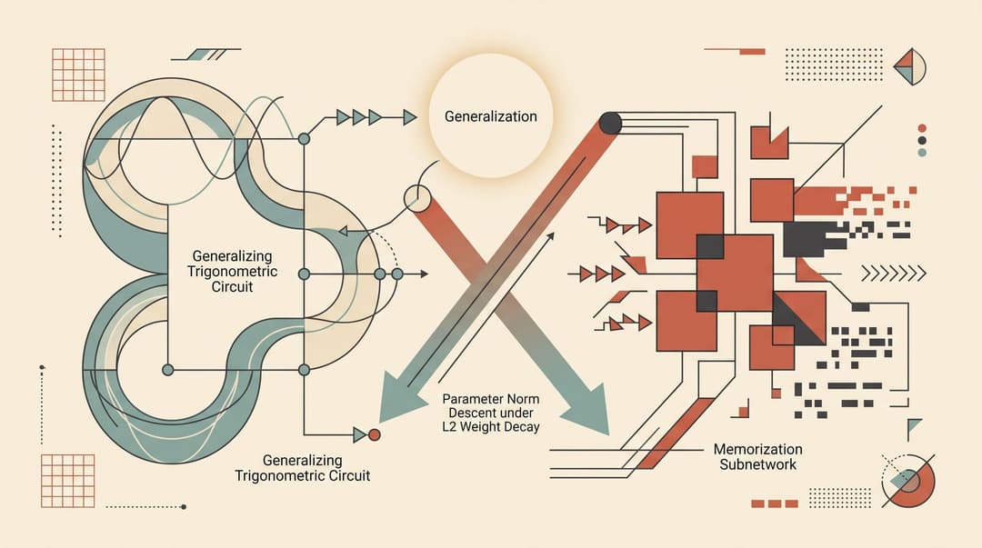
This phenomenon, termed grokking or delayed generalization, challenged conventional understanding of overfitting, regularization, and model convergence. Subsequent mechanistic interpretability and loss landscape research has revealed that grokking is not an anomaly, but the macroscopic signature of microscopic competition between distinct internal subnetworks: a rapidly learned, high-norm memorization circuit and a slower-learning, highly efficient generalizing circuit.

Understanding grokking provides deep insights into how overparameterized neural networks, including large language models, transition from surface-level pattern matching to robust algorithmic reasoning during extended training.

1. The Discovery of Delayed Generalization

The grokking phenomenon was first systematically documented by Power et al. (2022) at OpenAI. The researchers trained small, standard decoder-only Transformer models on binary algorithmic operations over finite fields, such as modular addition ($a + b \pmod p$), modular subtraction, modular division, and permutation composition.

When evaluating a model trained on a subset of the multiplication or addition table for a prime modulus such as $p = 97$, the training trajectory exhibited a distinct pattern:

1. Immediate Memorization (0 to 1,000 optimization steps): Training accuracy surged to 100%, and training loss dropped toward zero. Validation accuracy remained at the random guess baseline (around $1/p \approx 1\%$).
2. The Generalization Plateau (1,000 to 50,000+ optimization steps): Training accuracy remained locked at 100%. Validation accuracy remained near 0%, and validation loss frequently climbed, suggesting severe overfitting under traditional early-stopping criteria.
3. The Abrupt Phase Transition (50,000 to 100,000 steps): Validation accuracy spiked from chance level to 100% over a very narrow training interval, while training performance remained unchanged.

Power et al. demonstrated that this delayed generalization required substantial weight decay ($L_2$ regularization) and was sensitive to dataset size: smaller training fractions required exponentially more optimization steps before the validation transition occurred.

2. The Mechanistic Anatomy: Fourier Circuits and Trigonometric Identities

To understand why validation accuracy remains flat while the network continues to train, Nanda et al. (2023) performed a mechanistic interpretability analysis on a 1-layer Transformer trained on modular addition ($a + b \pmod p$).

Instead of maintaining a massive lookup table of memorized input pairs, the fully generalized network discovered an elegant mathematical algorithm based on the Discrete Fourier Transform (DFT) and trigonometric angle addition identities:

$$\cos(\omega (a + b)) = \cos(\omega a)\cos(\omega b) - \sin(\omega a)\sin(\omega b)$$ $$\sin(\omega (a + b)) = \sin(\omega a)\cos(\omega b) + \cos(\omega a)\sin(\omega b)$$

The reverse-engineered circuit operates through four distinct computational stages:

Step 1: Embedding via Circular Projections

The embedding matrix maps discrete token indices $a$ and $b$ to continuous representations. Rather than arbitrary random vectors, the trained embedding matrix projects inputs onto circular orbits corresponding to a sparse set of key spatial frequencies $\omega_k = \frac{2\pi k}{p}$, embedding $\cos(\omega_k a)$ and $\sin(\omega_k a)$.

Step 2: Attention Head Routing

The single attention layer passes both token representations to the MLP layer, preserving the trigonometric coordinates across the residual stream.

Step 3: Quadratic Multi-Layer Perceptron (MLP) Activation

The MLP activation function approximates quadratic terms (e.g. via ReLU or GELU non-linearities). When presented with linear combinations of trigonometric embeddings, the quadratic expansion computes terms of the form:

$$(\cos(\omega a) + \cos(\omega b))^2 = \cos^2(\omega a) + \cos^2(\omega b) + 2\cos(\omega a)\cos(\omega b)$$

By combining these crossed products, the MLP calculates $\cos(\omega(a+b))$ and $\sin(\omega(a+b))$ directly from the separate inputs $a$ and $b$.

Step 4: Unembedding and Logit Extraction

The unembedding matrix acts as an inverse Fourier transform. By multiplying the resulting latent vector by directional vectors corresponding to each candidate output token $c \in \{0, \dots, p-1\}$, the dot product produces maximum logit values precisely when $c \equiv a + b \pmod p$.

Nanda et al. introduced progress measures (such as the Fourier gap and excluded loss), demonstrating that the internal Fourier circuit grows steadily and continuously throughout the entire plateau phase, long before validation accuracy registers any change.

3. The Three-Phase Model of Grokking Dynamics

Mechanistic analysis shows that grokking unfolds in three distinct continuous phases:

[Phase 1: Memorization] ──> [Phase 2: Circuit Formation] ──> [Phase 3: Cleanup / Pruning]
  • High parameter norm       • Generalizing Fourier          • Weight decay penalizes
  • Training loss -> 0          features emerge in background   memorization weights
  • Test accuracy = ~1%       • Dual circuits coexist         • Test accuracy -> 100%

Phase 1: Memorization

The network uses its high-dimensional parameter capacity to memorize the training data. Because memorizing independent data points requires minimal cross-sample coordination, gradient descent finds memorization solutions quickly. However, this brute-force lookup relies on independent, unaligned weight vectors across many parameters, resulting in a large total parameter norm $\|W\|_2$.

Phase 2: Circuit Formation

As training continues, gradient updates begin reinforcing shared patterns across training examples. The structured Fourier circuit begins to form. During this stage, the model relies on a composite strategy: predictions are driven partly by memorization weights and partly by embryonic generalizing features. Because validation samples share the underlying algebraic structure but lack memorized sample points, validation loss remains high.

Phase 3: Cleanup and Parameter Reallocation

Under $L_2$ weight decay, the optimization objective is:

$$\mathcal{L}_{\text{total}}(W) = \mathcal{L}_{\text{task}}(W) + \frac{\lambda}{2} \|W\|_2^2$$

A structured generalizing circuit is vastly more parameter-efficient than a lookup table: a handful of Fourier frequencies can represent all $p^2$ modular combinations using small, coherent weights. Once the generalizing circuit generates sufficiently confident logits to satisfy the task loss $\mathcal{L}_{\text{task}}$, weight decay aggressively drives the unshared memorization weights toward zero. The network purges the memorization subnetwork, and validation accuracy surges to 100%.

4. Theory of Circuit Efficiency

Formalizing this multi-circuit dynamic, Varma et al. (2023) introduced the Theory of Circuit Efficiency. They defined the efficiency of a subnetwork $C$ as the magnitude of logits it produces on dataset $\mathcal{D}$ per unit of parameter norm:

$$\text{Efficiency}(C) = \frac{\mathbb{E}_{x \in \mathcal{D}} [\text{logit}_C(x)]}{\|W_C\|_2}$$

Varma et al. showed that:

1. Memorizing circuits ($C_{\text{mem}}$) have high initial learning speed because their gradient signal is unconstrained by global structure, but their efficiency decreases as the training dataset size increases. To memorize $N$ distinct points, $C_{\text{mem}}$ requires weight norm scaling roughly proportional to $\sqrt{N}$.
2. Generalizing circuits ($C_{\text{gen}}$) have slower initial learning speed due to complex multi-layer feature alignment, but their parameter norm is independent of dataset size ($O(1)$ scaling).

Circuit Efficiency Comparison:
• Memorization Circuit (C_mem): Fast learning rate, poor norm efficiency (O(sqrt(N)) norm cost)
• Generalizing Circuit (C_gen): Slow learning rate, high norm efficiency (O(1) norm cost)
• Critical Threshold: Grokking occurs when N > N_critical, making C_gen the global minimum under weight decay.

This formulation revealed the existence of a critical dataset size ($N_{\text{crit}}$). Below $N_{\text{crit}}$, memorization is more norm-efficient, and the model never groks. Above $N_{\text{crit}}$, generalization represents the unique global minimum of the regularized loss landscape, making grokking inevitable if optimization runs long enough.

The theory accurately predicted novel empirical behaviors:

• Ungrokking: When the regularization penalty or dataset composition is modified after convergence, a generalizing network can spontaneously decay back into an overfitted memorization state.
• Semi-Grokking: On multi-task or hierarchical objectives, models can exhibit staged, partial grokking transitions corresponding to individual sub-circuits reaching critical efficiency at different step counts.

5. Regularization, Loss Landscapes, and the Slingshot Mechanism

While algorithmic datasets provide clean mathematical testbeds, researchers have demonstrated that grokking occurs across standard deep learning architectures and domains:

• Omnigrok on Standard Datasets: Liu et al. (2022) demonstrated that grokking readily occurs on MNIST, CIFAR-10, and language modeling benchmarks when networks are initialized with large initial weight norms or trained under specific regularization schedules.
• Adaptive Optimizers and the Slingshot Mechanism: Thilak et al. (2022) analyzed how optimizers like AdamW interact with loss surface geometry. When weight decay pushes weights toward the origin, the network enters an unstable, highly curved region of the loss surface. The resulting gradient spikes launch the optimizer out of sharp memorization valleys and catapult it into wider, flatter generalizing basins.

Loss Landscape Transition:
[Sharp Memorization Basin] ──(Weight Decay + Gradient Spikes)──> [Flat Generalizing Minimum]
  • High Hessian trace                                              • Low Hessian trace
  • Poor out-of-distribution stability                             • High architectural robustness

6. Implications for Large Language Models and AI Pre-Training

The mechanistic mechanics of grokking offer fundamental lessons for training modern foundation models and understanding LLM reasoning:

1. The Reality of Overtraining and Compute-Optimal Frontiers

Historically, training was halted when validation loss plateaued to prevent overfitting. Modern LLM training regimens (such as LLaMA and subsequent open-weight foundation models) routinely train models on tens of trillions of tokens, well beyond the traditional compute-optimal Chinchilla frontier. Extended training under weight decay allows models to continuously compress memorized facts into compact, generalizable reasoning circuits.

2. Discontinuous Capabilities vs. Smooth Internal Progress

The sudden appearance of capabilities (such as multi-step arithmetic, in-context translation, or symbolic reasoning) is often cited as evidence of unpredictable emergent abilities. Mechanistic grokking studies demonstrate that internal circuit formation is smooth and continuous. The apparent discontinuity is an artifact of non-linear performance metrics (like exact-match accuracy) that remain near zero until the underlying circuit surpasses a specific confidence threshold.

3. Safety and Alignment Circuit Stability

The observation of "ungrokking" highlights that model alignment and safety guardrails, when trained via fine-tuning or RLHF, function as competing circuits against pre-trained base distributions. Understanding circuit efficiency ensures that safety constraints are trained with sufficient data volume and regularization to achieve permanent, stable circuit dominance.

Sources

• Power, A., Burda, Y., Edwards, H., Babuschkin, I., & Misra, V. (2022). Grokking: Generalization Beyond Overfitting on Small Algorithmic Datasets. arXiv: 2201.02177
• Nanda, N., Chan, L., Lieberum, T., Smith, J., & Steinhardt, J. (2023). Progress Measures for Grokking via Mechanistic Interpretability. ICLR 2023. arXiv: 2301.05217
• Varma, V., Shah, R., Kenton, Z., Kramár, J., & Kumar, R. (2023). Explaining Grokking Through Circuit Efficiency. arXiv: 2309.02390
• Liu, Z., Kitouni, O., Nolte, N., Michaud, E. J., Tegmark, M., & Williams, M. (2022). Towards Understanding Grokking: An Effective Theory of Representation Learning (Omnigrok). arXiv: 2210.01117
• Thilak, V., Littwin, E., Zhai, S., Saremi, O., Paiss, R., & Susskind, J. (2022). The Slingshot Mechanism: An Empirical Study of Adaptive Optimizers and the Grokking Phenomenon. arXiv: 2206.04817