Arithmetic Intensity and the Roofline Model in Large Language Models: Why Generation Is Memory-Bound and Prefill Is Compute-Bound

Every optimization in modern large language model (LLM) serving exists to solve a single hardware reality: running a Transformer model is not one computational problem, but two completely distinct workloads operating on opposite sides of a physical performance barrier.

When an LLM processes a prompt during the prefill phase, it saturates modern GPU Tensor Cores, operating near theoretical peak floating-point throughput. When that same model generates subsequent tokens autoregressively during the decode phase, GPU compute utilization plummets to single-digit percentages, leaving trillions of arithmetic operations per second idle while the processor waits for memory access.

Understanding this divergence requires analyzing hardware execution through the lens of the Roofline Model and arithmetic intensity.

The Roofline Model and Arithmetic Intensity

First formalized by Samuel Williams, Andrew Waterman, and David Patterson in 2009, the Roofline Model provides an intuitive visual bound relating an application's execution performance to two fundamental hardware constraints:

1. Peak Computational Performance ($P_{\text{peak}}$): The maximum rate of floating-point operations the processor execution units can sustain (measured in FLOP/s or TFLOP/s).
2. Peak Memory Bandwidth ($B_{\text{mem}}$): The maximum rate at which data can be transferred from high-bandwidth memory (HBM) into on-chip SRAM, registers, and execution caches (measured in Bytes/s or TB/s).

The parameter connecting an algorithm to these physical ceilings is operational intensity (commonly called arithmetic intensity), defined as the ratio of arithmetic operations performed to bytes of data moved across the memory bus:

$$I = \frac{\text{Floating-Point Operations (FLOPs)}}{\text{DRAM Bytes Transferred (Bytes)}}$$

The Roofline Model establishes that maximum attainable performance ($P_{\text{attainable}}$) is the minimum of these two bounds:

$$P_{\text{attainable}} = \min(P_{\text{peak}}, I \times B_{\text{mem}})$$

Performance (TFLOP/s)
  ^
  |                     +--------------------------- Peak Compute Ceiling (P_peak)
  |                    /
  |                   /  Compute-Bound Regime
  |                  /   (Tensor Cores Saturated)
  |                 /
  |                /
  |               /
  |              / 
  |             /
  |            /  Memory-Bound Regime
  |           /   (Memory Bandwidth Starvation)
  |          /
  |         /
  |        /
  |       /
  |      +
  +------+------------------------------------------> Arithmetic Intensity (FLOP/Byte)
         ^
      Ridge Point (I_ridge = P_peak / B_mem)

The intersection where the memory bandwidth ceiling meets the peak compute ceiling is the ridge point ($I_{\text{ridge}}$):

$$I_{\text{ridge}} = \frac{P_{\text{peak}}}{B_{\text{mem}}}$$

Any algorithm whose arithmetic intensity falls below $I_{\text{ridge}}$ is strictly memory bandwidth-bound. Increasing compute capability (e.g., faster Tensor Cores) yields zero speedup for memory-bound workloads because execution time is entirely dominated by data transfer latency. Conversely, workloads with arithmetic intensity above $I_{\text{ridge}}$ are compute-bound, where the memory bus supplies data faster than execution units can consume it.

Hardware Ridge Points on Modern Accelerators

Over the past decade, processor computational speed has scaled at a much faster rate than memory bandwidth, a dynamic widely known as the "memory wall." Consequently, modern accelerator architectures feature high ridge points.

Consider the specifications for prominent data center AI accelerators:

| Hardware Accelerator | Precision | Peak Compute ($P_{\text{peak}}$) | HBM Bandwidth ($B_{\text{mem}}$) | Hardware Ridge Point ($I_{\text{ridge}}$) | | :--- | :--- | :--- | :--- | :--- | | NVIDIA A100 SXM4 (80GB) | FP16 Dense | 312 TFLOP/s | 2.039 TB/s | 153.0 FLOP/Byte | | NVIDIA H100 SXM5 (80GB) | FP16 Dense | 989.5 TFLOP/s | 3.35 TB/s | 295.4 FLOP/Byte | | NVIDIA H100 SXM5 (80GB) | FP8 Dense | 1,979.0 TFLOP/s | 3.35 TB/s | 590.7 FLOP/Byte | | Google TPU v4 | BF16 Dense | 275 TFLOP/s | 1.20 TB/s | 229.2 FLOP/Byte | | NVIDIA B200 (Blackwell) | FP16 Dense | 2,250 TFLOP/s | 8.00 TB/s | 281.3 FLOP/Byte | | NVIDIA B200 (Blackwell) | FP8 Dense | 4,500 TFLOP/s | 8.00 TB/s | 562.5 FLOP/Byte |

On an NVIDIA H100 SXM5 GPU executing FP16 operations, any kernel requiring fewer than 295.4 FLOPs for every byte transferred from HBM is memory-bandwidth bound. For FP8 computation, the ridge point doubles to 590.7 FLOP/Byte.

The Prefill Phase: Matrix-Matrix Multiplication (GEMM)

During the initial prefill (prompt processing) phase, the model receives a prompt of length $T_{\text{in}}$ tokens. Because the entire prompt is known in advance, the model processes all $T_{\text{in}}$ tokens in parallel.

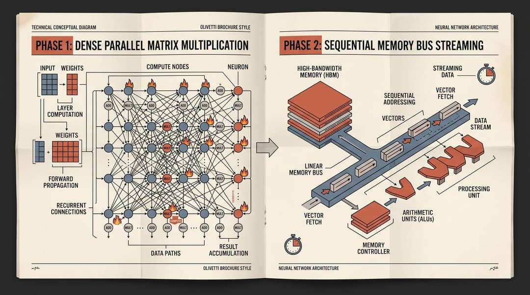
In each Transformer layer, the linear projections (Query, Key, Value, Output, and MLP projections) perform general matrix-matrix multiplications (GEMM). For an input activation tensor $X \in \mathbb{R}^{B \times T_{\text{in}} \times d_{\text{model}}}$ and a weight matrix $W \in \mathbb{R}^{d_{\text{model}} \times d_{\text{out}}}$:

1. Floating-point operations: Computing $Y = XW$ requires $2 \times B \times T_{\text{in}} \times d_{\text{model}} \times d_{\text{out}}$ FLOPs (one multiply and one add per element).
2. Memory transfers: Assuming weights are loaded once from HBM into SRAM and activations are streamed, the total bytes loaded are $(2 \times d_{\text{model}} \times d_{\text{out}}) + (2 \times B \times T_{\text{in}} \times d_{\text{model}})$ bytes for FP16 (2 bytes per element).

When $B \times T_{\text{in}}$ is large (e.g., a batch of 8 requests with 2,048 prompt tokens each, so $B \times T_{\text{in}} = 16,384$), the weight loading term is amortized across thousands of token vectors:

$$I_{\text{prefill}} \approx \frac{2 \times (B \cdot T_{\text{in}}) \times d_{\text{model}} \times d_{\text{out}}}{2 \times d_{\text{model}} \times d_{\text{out}}} = B \cdot T_{\text{in}} \text{ FLOP/Byte}$$

With $B \cdot T_{\text{in}} = 16,384$, the arithmetic intensity reaches thousands of FLOPs per byte, far exceeding the H100's ridge point of 295.4 FLOP/Byte.

As documented by Pope et al. (2022) and Sheng et al. (2023), prefill execution operates at or near peak Model FLOPs Utilization (MFU), typically achieving 50% to 75% of hardware maximum throughput. The execution time during prefill scales with total token count and computational complexity rather than memory bus bandwidth.

The Decode Phase: Matrix-Vector Multiplication (GEMV)

Once prompt prefill completes, autoregressive text generation begins. Autoregressive models generate tokens strictly one at a time because each new token $y_t$ depends causally on all preceding tokens:

$$y_t \sim P(y_t \mid x_1, \dots, x_{T_{\text{in}}}, y_1, \dots, y_{t-1})$$

In a single-request scenario ($B=1$), generating token $t$ requires passing a single token activation vector $x_t \in \mathbb{R}^{1 \times d_{\text{model}}}$ through the entire network. The operations across all linear layers are no longer matrix-matrix multiplications (GEMM); they degenerate into matrix-vector multiplications (GEMV).

The Arithmetic Intensity of Batch-Size-1 Generation

Consider a model with $P$ parameters stored in FP16 (16 bits = 2 bytes per parameter). To compute a single forward pass for $T=1$:

1. Floating-point operations: A standard forward pass requires approximately $2P$ FLOPs per token (2 FLOPs per parameter for matrix multiplications).
2. Weight memory transfers: To multiply the single input vector by the weight matrices, every single weight in the model must be loaded from HBM across the memory bus into on-chip registers. This requires $2P$ bytes of memory transfer.

Calculating the resulting arithmetic intensity for the model's feedforward and projection weights:

$$I_{\text{decode}} = \frac{\text{Compute}}{\text{Memory Traffic}} \approx \frac{2P \text{ FLOPs}}{2P \text{ Bytes}} = 1.0 \text{ FLOP/Byte}$$

On an NVIDIA H100 GPU with a ridge point of 295.4 FLOP/Byte, an arithmetic intensity of $1.0\text{ FLOP/Byte}$ means the hardware operates at:

$$\text{Efficiency} = \frac{1.0}{295.4} \approx 0.34\% \text{ of Peak Compute}$$

More than 99.6% of the GPU's theoretical compute capacity sits completely idle, stalled waiting for HBM to stream parameters over the internal bus.

+-----------------------------------------------------------------------------+
| LLM Serving Phase Comparison (H100 SXM5, FP16)                             |
+-----------------------------------------------------------------------------+
| Phase    | Primary Kernel | Batch Size | Arithmetic Intensity | Regime      |
+----------+----------------+------------+----------------------+-------------+
| Prefill  | GEMM           | B * T >> 1 | > 1,000 FLOP/Byte    | Compute     |
| Decode   | GEMV           | B = 1      | ~ 1.0 FLOP/Byte      | Memory-Bound|
+-----------------------------------------------------------------------------+

The KV Cache Memory Bandwidth Overhead

The memory bandwidth bottleneck during token generation is not limited to model weights; it is compounded by the Key-Value (KV) cache.

To avoid recomputing keys and values for all historical tokens at every step, inference engines store the key and value projections from previous tokens in GPU memory. During each decoding step, the new query vector $q_t$ must attend to all previous key vectors and compute a weighted sum over all value vectors.

For a sequence of length $S$ with $L$ layers, $N_{\text{kv}}$ key-value heads, and head dimension $d_{\text{head}}$, the total KV cache size per request is:

$$\text{KV Size (Bytes)} = 2 \times 2 \times L \times N_{\text{kv}} \times d_{\text{head}} \times S$$

At each decoding step $t$:

• The GPU must read the entire accumulated KV cache from HBM into SRAM to compute multi-head attention.
• The GPU must write the newly generated key and value vectors ($4 \times L \times N_{\text{kv}} \times d_{\text{head}}$ bytes) back to HBM.

As sequence length $S$ grows into tens or hundreds of thousands of tokens, the bytes transferred for KV cache retrieval can surpass the bytes loaded for model weights. This further depresses effective arithmetic intensity and establishes sequence length as a primary throughput constraint.

Architectural Mechanisms to Overcome the Memory Wall

Because autoregressive decoding is constrained by memory bandwidth rather than compute limits, every major software and architectural innovation in modern LLM serving targets increasing arithmetic intensity or reducing bytes moved across the memory bus:

                  +---------------------------------------------------+
                  | Strategies for Overcoming the Memory Wall         |
                  +---------------------------------------------------+
                                            |
        +-----------------------------------+-----------------------------------+
        |                                                                       |
+-------v-----------------------+                                       +-------v-----------------------+
|  Increase Arithmetic Intensity|                                       |  Reduce Bytes Transferred     |
+-------------------------------+                                       +-------------------------------+
| * Continuous Batching (B > 1) |                                       | * Weight Quantization (W4A16) |
| * Speculative Decoding        |                                       | * KV Cache Quantization (FP8) |
| * Multi-Token Prediction (MTP)|                                       | * GQA / MQA / MLA Head Sharing|
+-------------------------------+                                       +-------------------------------+

1. Continuous and Dynamic Batching

By grouping $B$ independent user requests into a single forward pass, the model weights loaded from HBM are multiplied against $B$ token vectors simultaneously. This converts GEMV back into a small GEMM, scaling arithmetic intensity roughly linearly with batch size ($I \approx B \text{ FLOP/Byte}$) until the batch size approaches the hardware ridge point ($B \approx 300$). As demonstrated by Yu et al. (2022) in Orca, iteration-level scheduling prevents request completion mismatches from causing pipeline bubbles.

2. Weight and KV Cache Quantization

Quantizing model weights from FP16 (16 bits) to INT4 or FP4 (4 bits) reduces weight data traffic by 75%. Because generation latency at small batch sizes is governed directly by memory bandwidth:

$$\text{Time per Token} \approx \frac{\text{Model Bytes Loaded}}{\text{Memory Bandwidth}}$$

Halving the precision of model weights doubles token generation speed on memory-bound workloads, even if the dequantization overhead slightly increases arithmetic instructions.

3. Key-Value Head Compression (GQA, MQA, and MLA)

Standard Multi-Head Attention maintains separate Key and Value heads for every Query head ($N_{\text{kv}} = N_{\text{heads}}$). Grouped-Query Attention (GQA) shares single Key and Value heads across groups of Query heads, cutting KV cache memory traffic by 4x to 8x. Multi-Head Latent Attention (MLA) compresses Key-Value projections into a low-rank latent vector, slashing KV cache memory transfers by up to 93%.

4. Speculative Decoding

Speculative decoding uses a compact, fast draft model to speculate $K$ candidate tokens. The primary target model then verifies all $K$ tokens in a single forward pass using GEMM. If multiple tokens are accepted, the target model processes $K$ tokens for the memory cost of loading its weights once, effectively boosting generation arithmetic intensity by a factor proportional to the mean acceptance rate.

5. Disaggregated Prefill and Decode Architectures

Because prefill and decode exhibit opposing resource bottlenecks, co-locating them on the same GPU creates destructive interference: compute-heavy prefill operations preempt memory-bandwidth-sensitive decode streams, introducing severe latency spikes (time-to-first-token versus inter-token latency trade-offs). Disaggregated serving architectures such as Splitwise partition GPU clusters into dedicated prefill pools (optimized for high TFLOP/s) and decode pools (optimized for maximum memory bandwidth and high interconnect speeds), transferring intermediate KV caches across high-speed networks.

Summary

The Roofline Model provides the foundational mathematical framework explaining why large language model inference behaves as two fundamentally different computational tasks:

• Prefill is Compute-Bound: Parallel processing across entire input sequences yields high arithmetic intensity ($I > I_{\text{ridge}}$), saturating Tensor Cores and achieving high Model FLOPs Utilization.
• Decode is Memory-Bound: Sequential, token-by-token generation forces full model weight streaming per forward pass, resulting in near-unity arithmetic intensity ($I \approx 1.0\text{ FLOP/Byte}$) that leaves modern execution engines starved for data.

Understanding the roofline curve makes clear why serving system optimizations focus relentlessly on memory footprint reduction, batch consolidation, speculative verification, and phase disaggregation: until hardware memory bandwidth catches up to arithmetic capacity, generation performance will remain bounded by the memory bus.

Sources

• Williams, S., Waterman, A., & Patterson, D. (2009). Roofline: An Insightful Visual Performance Model for Multicore Architectures. Communications of the ACM, 52(4), 65–76. ACM Digital Library
• Pope, R., Douglas, S., Chowdhery, A., Devlin, J., Bradbury, J., Levskaya, A., Heek, J., Xiao, K., Agrawal, S., & Dean, J. (2022). Efficiently Scaling Transformer Inference. arXiv:2211.05102. arXiv
• Patel, P., Choukse, E., Zhang, C., Shah, A., & Goiri, Í. (2023). Splitwise: Efficient Generative LLM Serving Using Phase Splitting. arXiv:2311.18677. arXiv
• Sheng, Y., Zheng, L., Yuan, B., Li, Z., Ryabinin, M., Fu, D. Y., Xie, C. X., Chen, B., Barrett, C., & Ré, C. (2023). FlexGen: High-Throughput Generative Inference of Large Language Models with a Single GPU. arXiv:2303.06865. arXiv
• Yu, G. I., Jeong, J. S., Kim, G. W., Kim, S., & Chun, B. G. (2022). Orca: A Distributed Serving System for Transformer-Based Generative Models. USENIX OSDI '22. USENIX
• Ainslie, J., Ontanon, S., Alberti, C., Cvicek, V., Fisher, Z., Pham, P., Ravula, A., Sumbaly, S., & Yang, L. (2023). GQA: Training Generalized Multi-Query Transformer Models from Multi-Head Checkpoints. arXiv:2305.13245. arXiv
• DeepSeek-AI. (2024). DeepSeek-V2: A Strong, Economical, and Efficient Mixture-of-Experts Language Model. arXiv:2405.04434. arXiv
• Leviathan, Y., Kalman, M., & Matias, Y. (2023). Fast Inference from Transformers via Speculative Decoding. arXiv:2211.17192. arXiv