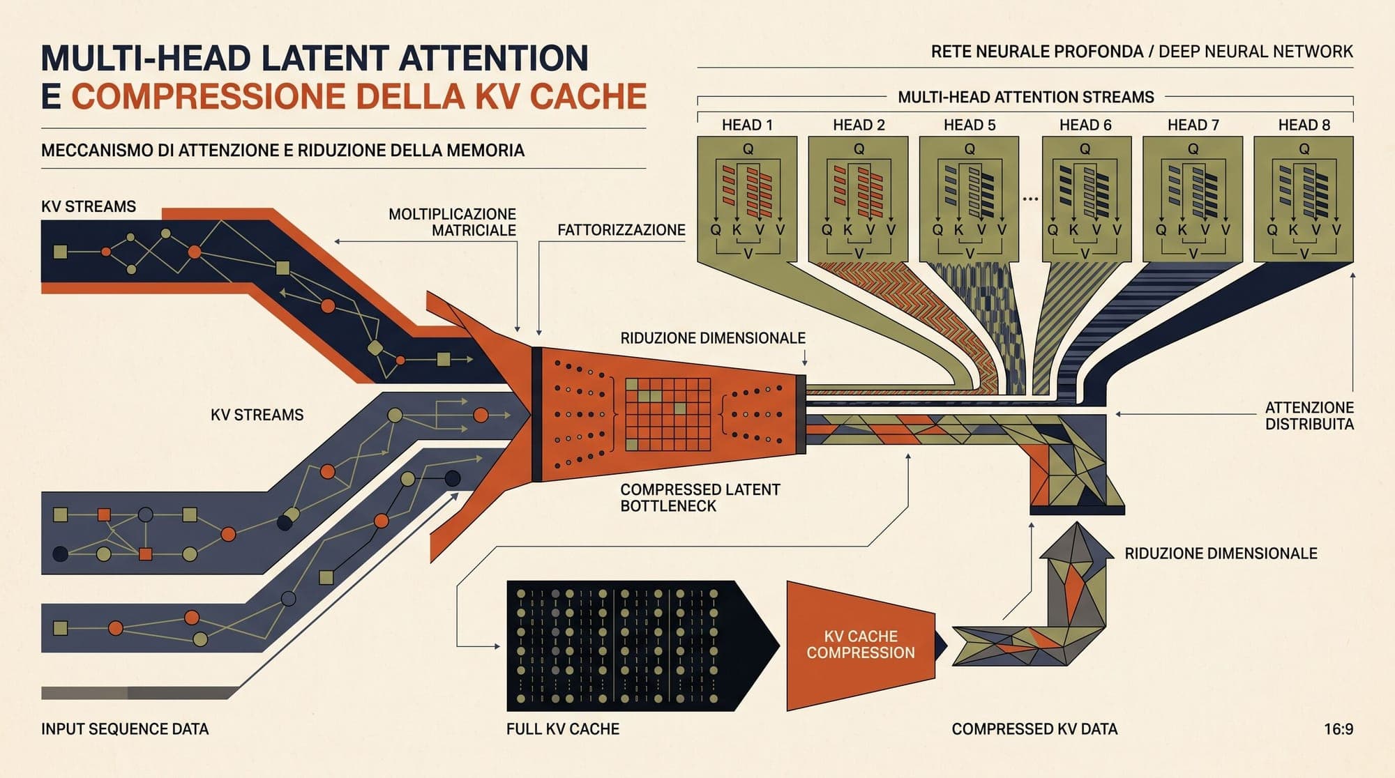
Multi-Head Latent Attention (MLA): Mathematical Foundations, Low-Rank KV Compression, Decoupled RoPE Mechanics, and Matrix Absorption

Autoregressive inference in large language models is fundamentally constrained by memory bandwidth rather than floating-point computation throughput. During the generation phase, the transformer must load the Key-Value (KV) cache of all prior tokens from high-bandwidth memory (HBM) to on-chip SRAM for every newly generated token. As context lengths scale to hundreds of thousands of tokens and concurrent batch sizes increase, the aggregate memory footprint and memory access overhead of the KV cache dominate serving economics.

Multi-Head Latent Attention (MLA), introduced by DeepSeek-AI (2024) in the DeepSeek-V2 and DeepSeek-V3 architectures, restructures the attention mechanism by projecting Keys and Values into a low-rank compressed latent space. By combining low-rank projection with a decoupled positional embedding mechanism, MLA allows serving engines to cache only compressed latent representations while mathematically absorbing the up-projection matrices directly into the Query and Output projections during generation. This reduces the inference-time KV cache footprint by over 93% compared to standard Multi-Head Attention (MHA) while matching or exceeding the expressivity of full-rank MHA.

1. The Memory-Bandwidth Wall in Transformer Decoding

In autoregressive token generation, the model predicts token t + 1 given past tokens 1, ..., t. While the feedforward (FFN/MoE) projections require processing only the single current hidden state h_t in R^d, the attention layer must compute cross-attention against the entire historical context:

Attention(Q_t, K_<=t, V_<=t) = softmax( (Q_t * K_<=t^T) / sqrt(d_h) ) * V_<=t

The arithmetic intensity of this step, defined as the ratio of floating-point operations (FLOPs) to memory transactions (Bytes transferred), drops precipitously during decoding. For a sequence of length S, computing attention logits requires O(S * d) FLOPs while transferring O(S * d) bytes of KV cache from HBM. On modern accelerator architectures such as NVIDIA H100 (which delivers 1,979 TFLOPS of FP16 tensor core compute against 3.35 TB/s of HBM3 bandwidth), memory bus saturation occurs when arithmetic intensity falls below approximately 590 FLOPs/byte. Consequently, standard autoregressive decoding operates in a strictly memory-bound regime.

+-----------------------------------------------------------------------------------+
|                        Standard KV Cache Memory Footprint                         |
|                                                                                   |
|  Memory per Token = 2 * n_layers * n_heads * d_head * b (bytes)                   |
|                                                                                   |
|  For a 60-layer model (128 heads, d_head = 128, FP16 precision b = 2):            |
|  Memory per token = 2 * 60 * 128 * 128 * 2 = 3,932,160 bytes (~3.93 MB / token)   |
|  At 128k context length: 3.93 MB * 131,072 = 515.4 GB per active sequence         |
+-----------------------------------------------------------------------------------+

Prior approaches to KV cache compression introduced architectural trade-offs:

• Multi-Query Attention (MQA): Introduced by Shazeer (2019), MQA collapses the number of Key and Value heads to 1, sharing a single Key-Value head across all Query heads. This reduces the KV cache by a factor of n_heads, but severely restricts model capacity and retrieval fidelity across disparate subspaces.
• Grouped-Query Attention (GQA): Proposed by Ainslie et al. (2023), GQA groups Query heads into G partitions (1 < G < n_heads), with each group sharing one KV head. While GQA serves as a practical compromise adopted in Llama 3 and Mistral, the reduction factor is bounded by n_heads / G, and expressive degradation emerges at high compression ratios.

2. Standard Multi-Head Attention Formulations

In standard Multi-Head Attention (MHA), let d denote the hidden dimension, n_h the number of attention heads, and d_h the per-head dimension (d = n_h * d_h). For input hidden state h_t in R^d at position t:

• q_t = [q_{t,1}; q_{t,2}; ...; q_{t,n_h}] = W^Q * h_t
• k_t = [k_{t,1}; k_{t,2}; ...; k_{t,n_h}] = W^K * h_t
• v_t = [v_{t,1}; v_{t,2}; ...; v_{t,n_h}] = W^V * h_t

where W^Q, W^K, W^V are in R^{(n_h * d_h) x d}. For head i in {1, ..., n_h}, the projected head vectors are q_{t,i}, k_{t,i}, v_{t,i} in R^{d_h}.

Under Rotary Position Embedding (Su et al., 2021), positional information is injected by multiplying Query and Key representations by a block-diagonal orthogonal rotation matrix R_t in R^{d_h x d_h}:

• q_{t,i}^R = R_t * q_{t,i}
• k_{t,i}^R = R_t * k_{t,i}

The attention output for head i is computed as:

u_{t,i} = SUM_{j=1}^t softmax_j( ( (q_{t,i}^R)^T * k_{j,i}^R ) / sqrt(d_h) ) * v_{j,i}

The multi-head output combines all heads through output projection matrix W^O in R^{d x (n_h * d_h)}:

• o_t = W^O * [u_{t,1}; u_{t,2}; ...; u_{t,n_h}]

Under MHA, the serving system must cache the full tensor k_{j,i}^R and v_{j,i} for all layers, heads, and historical tokens j <= t.

3. Low-Rank Key-Value Joint Compression in MLA

Instead of directly projecting the hidden state h_t into separate per-head Key and Value tensors, Multi-Head Latent Attention compresses Keys and Values into a single low-rank latent vector c_t^{KV} in R^{d_c}, where the compression dimension d_c << n_h * d_h.

+-----------------------------------------------------------------------------------+
|                        MLA Low-Rank KV Compression Pipeline                       |
|                                                                                   |
|                                Input h_t in R^d                                   |
|                                       |                                           |
|                     Down-Projection Matrix W^{DKV} in R^{d_c x d}                 |
|                                       v                                           |
|                       Compressed Latent c_t^{KV} in R^{d_c}                       |
|                                  /         \                                      |
|                                 /           \                                     |
|    Up-Projection W^{UK} in R^{(n_h d_h) x d_c}  W^{UV} in R^{(n_h d_v) x d_c}     |
|              v                                             v                      |
|    Content Keys k_{t,i}^C in R^{d_h}             Content Values v_{t,i}^C in R^{d_v}|
+-----------------------------------------------------------------------------------+

Mathematically, the compression step is defined by down-projection matrix W^{DKV} in R^{d_c x d}:

• c_t^{KV} = W^{DKV} * h_t

From this shared latent representation c_t^{KV}, the uncompressed content Key vectors k_{t,i}^C and Value vectors v_{t,i}^C are generated via up-projection matrices W^{UK} in R^{(n_h * d_h) x d_c} and W^{UV} in R^{(n_h * d_v) x d_c}:

• [k_{t,1}^C; k_{t,2}^C; ...; k_{t,n_h}^C] = W^{UK} * c_t^{KV}
• [v_{t,1}^C; v_{t,2}^C; ...; v_{t,n_h}^C] = W^{UV} * c_t^{KV}

where d_v is the per-head Value dimension.

To reduce activation memory during training backpropagation, MLA also applies low-rank compression to the Query representations using down-projection matrix W^{DQ} in R^{d_c' x d} and up-projection matrix W^{UQ} in R^{(n_h * d_h) x d_c'}:

• c_t^Q = W^{DQ} * h_t
• [q_{t,1}^C; q_{t,2}^C; ...; q_{t,n_h}^C] = W^{UQ} * c_t^Q

where d_c' is the Query compression latent dimension.

4. The Non-Commutativity of RoPE and Matrix Projections

The fundamental obstacle to caching only the low-rank latent vector c_t^{KV} lies in the interaction between low-rank matrix decomposition and Rotary Position Embeddings (RoPE).

If RoPE were applied directly to the up-projected Key vectors k_{j,i}^C = W_{(i)}^{UK} * c_j^{KV}, the attention score between Query at position t and Key at position j would be:

Score_{t, j, i} = (q_{t,i})^T * ( R_{t-j} * ( W_{(i)}^{UK} * c_j^{KV} ) )

Because the rotary transformation R_{t-j} = R_t^T * R_j is position-dependent and sits strictly between the up-projection weight matrix W_{(i)}^{UK} and the Query vector, matrix multiplication associativity cannot be applied across time steps:

R_t^T * R_j * W_{(i)}^{UK} != W_{(i)}^{UK} * R_{t-j}

If position rotation is intertwined with the content Key, an inference engine would be forced to compute W_{(i)}^{UK} * c_j^{KV} and apply R_j dynamically for every past token j at every generation step t. This would require either materializing and caching the full uncompressed Keys in HBM (negating cache savings) or spending vast compute to recompute full-rank Keys on the fly at every step.

5. Decoupled Rotary Position Embedding (RoPE) Mechanics

To resolve this structural incompatibility, DeepSeek designed Decoupled RoPE. Rather than applying rotation to the full content Key and Query vectors, MLA partitions attention vectors into two decoupled pathways:

1. Content Pathway: Position-unaware (NoPE) vectors generated from low-rank latent projections (q_{t,i}^C and k_{t,i}^C).
2. Positional Pathway: A dedicated, low-dimensional rotary vector carrying RoPE (q_{t,i}^R and k_t^R).

Decoupled Key Formulation

The positional Key vector k_t^R in R^{d_R} is projected directly from hidden state h_t and rotated via RoPE:

• k_t^R = R_t * (W^{KR} * h_t)

where W^{KR} is in R^{d_R x d}. Crucially, the positional key k_t^R is shared across all attention heads (n_h), requiring only a single vector of dimension d_R (such as d_R = 64) per layer.

Decoupled Query Formulation

The positional Query vector q_{t,i}^R in R^{d_R} for head i is generated from the Query latent c_t^Q:

• q_{t,i}^R = R_t * (W_{(i)}^{QR} * c_t^Q)

where W_{(i)}^{QR} is in R^{d_R x d_c'}.

Unified Attention Score

The full Query and Key for head i are formed by concatenating the content and positional sub-vectors:

q_{t,i} = [q_{t,i}^C ; q_{t,i}^R]
k_{j,i} = [k_{j,i}^C ; k_j^R]

The resulting inner product expands as the sum of content and positional components:

q_{t,i}^T * k_{j,i} = (q_{t,i}^C)^T * k_{j,i}^C + (q_{t,i}^R)^T * k_j^R

The positional dot product (q_{t,i}^R)^T * k_j^R encapsulates relative position through standard RoPE properties:

(q_{t,i}^R)^T * k_j^R = (R_t * W_{(i)}^{QR} * c_t^Q)^T * (R_j * W^{KR} * h_j) = (W_{(i)}^{QR} * c_t^Q)^T * R_{j-t} * (W^{KR} * h_j)

Because k_{j,i}^C contains zero positional rotations, it can be expressed strictly as W_{(i)}^{UK} * c_j^{KV}.

6. Matrix Absorption (Absorb) Operation at Inference

Because the content Key up-projection W_{(i)}^{UK} contains no position-dependent operations, matrix multiplication associativity allows the up-projection to be mathematically absorbed into the Query vector before computing attention scores.

6.1 Query-Side Key Absorption

During autoregressive decoding, the content inner product is:

(q_{t,i}^C)^T * k_{j,i}^C = (q_{t,i}^C)^T * (W_{(i)}^{UK} * c_j^{KV}) = ((q_{t,i}^C)^T * W_{(i)}^{UK}) * c_j^{KV}

We define the transformed Query vector q~_{t,i}^C in R^{d_c}:

q~_{t,i}^C = (W_{(i)}^{UK})^T * q_{t,i}^C

The attention logit for head i at historical position j becomes:

Logit_{t, j, i} = ( (q~_{t,i}^C)^T * c_j^{KV} + (q_{t,i}^R)^T * k_j^R ) / sqrt(d_h + d_R)

In this form, the attention logit is computed directly between the transformed query q~_{t,i}^C and the cached latent vector c_j^{KV}. The full content Key tensor k_{j,i}^C in R^{n_h x d_h} is never materialized or stored in memory.

+-----------------------------------------------------------------------------------+
|                        Inference Matrix Absorption Flow                           |
|                                                                                   |
|  1. Attention Logit Computation:                                                  |
|     q_{t,i}^C in R^{d_h} ---> [ Multiply by (W_{(i)}^{UK})^T ] ---> q~_{t,i}^C in R^{d_c} |
|                                                                      |            |
|     Dot Product:  (q~_{t,i}^C)^T * c_j^{KV}  +  (q_{t,i}^R)^T * k_j^R             |
|                   \_______________________/     \___________________/             |
|                        Content Score               Positional Score               |
|                                                                                   |
|  2. Value Aggregation Computation:                                                |
|     Accumulate in latent space:  u~_{t,i} = SUM_j ( Attention_Score * c_j^{KV} )  |
|                                         |                                         |
|     Single output projection:    o_{t,i} = W_{(i)}^{UV} * u~_{t,i}                |
|     Combined with W^O:           o_t = SUM_i ( W_{(i)}^O * W_{(i)}^{UV} ) * u~_{t,i}|
+-----------------------------------------------------------------------------------+

6.2 Output-Side Value Absorption

Similarly, the attention output vector for head i is:

u_{t,i} = SUM_{j=1}^t A_{t,j,i} * v_{j,i}^C = SUM_{j=1}^t A_{t,j,i} * (W_{(i)}^{UV} * c_j^{KV})

where A_{t,j,i} = softmax_j(Logit_{t,j,i}). By linearity, W_{(i)}^{UV} can be factored out of the temporal summation:

u_{t,i} = W_{(i)}^{UV} * ( SUM_{j=1}^t A_{t,j,i} * c_j^{KV} ) = W_{(i)}^{UV} * u~_{t,i}

where u~_{t,i} = SUM_{j=1}^t A_{t,j,i} * c_j^{KV} in R^{d_c}.

The multi-head output projection accumulates these vectors:

o_t = SUM_{i=1}^{n_h} W_{(i)}^O * u_{t,i} = SUM_{i=1}^{n_h} (W_{(i)}^O * W_{(i)}^{UV}) * u~_{t,i}

We precompute the combined weight matrix W~_{(i)}^O = W_{(i)}^O * W_{(i)}^{UV} in R^{d x d_c}. The final attention output is:

o_t = SUM_{i=1}^{n_h} W~_{(i)}^O * u~_{t,i}

Under this formulation, the inference engine never expands or materializes v_{j,i}^C. The entire attention aggregation occurs over the d_c-dimensional latent representations.

7. Quantitative Comparison: Memory Footprint and Capacity

To evaluate the structural savings of MLA, we compare the per-token KV cache requirements across MHA, GQA, and MLA using the production hyperparameter configurations of DeepSeek-V2 and DeepSeek-V3 (L = 60 layers, n_h = 128 heads, d_h = 128, d_v = 128, d_c = 512, d_R = 64):

Per-Token Cache Memory Comparison

+---------------------------------------------------------------------------------------------+
| Architecture      | Elements Cached / Token / Layer | Bytes / Layer (FP16) | 128k Total Context |
+---------------------------------------------------------------------------------------------+
| Standard MHA      | 2 * 128 * 128 = 32,768          | 65,536 B (64.0 KB)   | 503.32 GB          |
| GQA (8 Groups)    | 2 *   8 * 128 =  2,048          |  4,096 B  (4.0 KB)   |  31.46 GB          |
| GQA (4 Groups)    | 2 *   4 * 128 =  1,024          |  2,048 B  (2.0 KB)   |  15.73 GB          |
| Multi-Query (MQA) | 2 *   1 * 128 =    256          |    512 B  (0.5 KB)   |   3.93 GB          |
| MLA (DeepSeek-V3) | d_c + d_R     =    576          |  1,152 B (1.125 KB)  |   8.85 GB          |
+---------------------------------------------------------------------------------------------+

MLA achieves a 98.24% reduction in KV cache memory compared to standard Multi-Head Attention, and consumes 71.88% less memory than an 8-group GQA setup.

KV Cache Memory per Active 128k Sequence (60 Layers):
MHA:   [==================================================] 503.3 GB
GQA-8: [===] 31.5 GB
GQA-4: [=] 15.7 GB
MLA:   [.] 8.85 GB

Expressivity and Rank Preservation

While GQA achieves cache reduction by forcing all Query heads within a group to share identical Key-Value projections in R^{d_h}, MLA preserves full multi-head expressivity. In MLA, each Query head maintains its own distinct projection matrix W_{(i)}^{UK} in R^{d_h x d_c}. Because d_c = 512 is substantially larger than an individual head dimension (d_h = 128), each head projects a distinct, non-degenerate subspace from the shared latent representation c^{KV}.

Empirical evaluations in the DeepSeek-V2 Technical Report (2024) and theoretical rank analyses (Gao et al., 2025) demonstrate that MLA matches the validation perplexity and downstream benchmark performance of standard full-rank MHA, outperforming both MQA and GQA baselines across equal parameter budgets.

8. Kernel-Level Execution: FlashMLA and Serving System Dynamics

Deploying MLA in high-throughput inference engines such as vLLM, SGLang, and DeepSeek's FlashMLA requires custom GPU attention kernels optimized for the dual-path logit computation.

+-----------------------------------------------------------------------------------+
|                        FlashMLA GPU Memory & Kernel Schedule                      |
|                                                                                   |
|  Global Memory (HBM3):                                                            |
|  [ Latent Cache c_j^{KV} (512 elems) ]   [ Positional Key k_j^R (64 elems) ]      |
|                      |                                      |                     |
|                      +------------------+-------------------+                     |
|                                         | Coalesced 576-element Memory Read       |
|                                         v                                         |
|  Streaming Multiprocessor (SRAM / Registers):                                     |
|  +-----------------------------------------------------------------------------+  |
|  | Chunked Matrix-Vector Core:                                                 |  |
|  | 1. Dot product: q~_{t,i}^C * c_j^{KV} (512-dim GEMV)                        |  |
|  | 2. Dot product: q_{t,i}^R * k_j^R     (64-dim GEMV)                         |  |
|  | 3. In-register Sum: Score = (Content_Dot + Pos_Dot) * scale                 |  |
|  | 4. Online Softmax Scaling & Latent Accumulation: u~_{t,i} += A * c_j^{KV}   |  |
|  +-----------------------------------------------------------------------------+  |
|                                         |                                         |
|                                         v                                         |
|  Output GEMM: o_t = SUM_i W~_{(i)}^O * u~_{t,i}                                   |
+-----------------------------------------------------------------------------------+

Kernel Optimization Mechanics:

• Coalesced Memory Access: The cached tensors c_j^{KV} in R^{512} and k_j^R in R^{64} are stored contiguously in memory as a single 576-element vector per token. This enables 128-bit aligned vector loads across GPU memory transactions.
• Online Softmax Scaling: Following FlashAttention principles (Dao et al., 2022), the kernel maintains running softmax normalizers m_t and l_t in registers while accumulating intermediate latent representations u~_{t,i} in R^{d_c}.
• Batch Size Scaling: Because the KV cache memory footprint is reduced by approximately 93%, serving engines can accommodate more than 5x larger decoding batch sizes within available GPU HBM, driving arithmetic intensity into the compute-bound regime and maximizing tensor core utilization.

9. Architectural Implications for Frontier Models

Multi-Head Latent Attention redefines the efficiency frontier of autoregressive sequence modeling. By decoupling position encodings from semantic content and exploiting matrix associativity, MLA eliminates the trade-off between memory footprint and multi-head representational capacity. As context windows expand beyond 100,000 tokens in agentic execution frameworks and long-horizon reasoning models, low-rank latent KV compression establishes a mathematically rigorous foundation for cost-effective inference serving.

Sources

• DeepSeek-AI. (2024). DeepSeek-V2: A Strong, Economical, and Efficient Mixture-of-Experts Language Model. arXiv:2405.04434.
• Liu, A., et al. (2024). DeepSeek-V3 Technical Report. arXiv:2412.19437.
• Su, J., Lu, Y., Pan, S., Murtadha, A., Bo, W., & Liu, Y. (2021). RoFormer: Enhanced Transformer with Rotary Position Embedding. arXiv:2104.09864.
• Shazeer, N. (2019). Fast Transformer Decoding: One Write-Head is All You Need. arXiv:1911.02150.
• Ainslie, J., et al. (2023). GQA: Training Generalized Multi-Query Transformer Models from Multi-Head Checkpoints. arXiv:2305.13245.
• Dao, T., Fu, D. Y., Ermon, S., Rudra, A., & Re, C. (2022). FlashAttention: Fast and Memory-Efficient Exact Attention with IO-Awareness. arXiv:2205.14135.
• Zhang, Y., et al. (2025). TransMLA: Multi-Head Latent Attention Is All You Need. arXiv:2502.07864.
• Gao, H., et al. (2025). A Random Matrix Theory Perspective on the Learning Dynamics of Multi-Head Latent Attention. arXiv:2507.09394.
• DeepSeek-AI. (2025). FlashMLA: Efficient Multi-Head Latent Attention Kernel for NVIDIA GPUs. GitHub Repository.