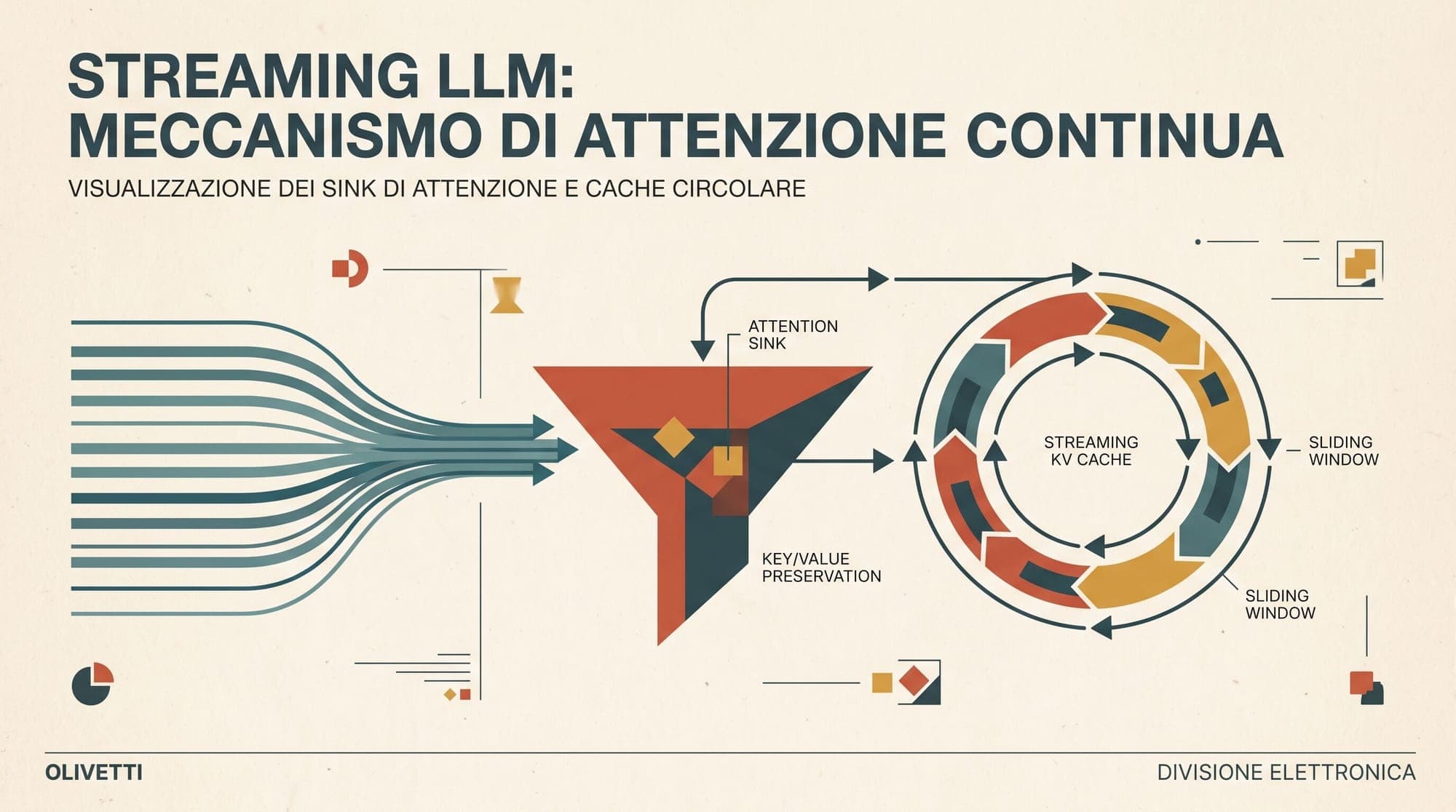
StreamingLLM and Attention Sinks: Mathematical Foundations of Softmax Normalization Artifacts, Initial Token Anchoring, and Infinite-Context Rolling KV-Cache Mechanics

In autoregressive Large Language Models (LLMs), long-context deployment is constrained by the quadratic compute complexity of attention and the linear memory growth of the Key-Value (KV) cache. For an LLM processing a sequence of length $L$ with batch size $b$, hidden dimension $d$, and $n_{kv}$ key-value heads across $N_L$ transformer layers, the aggregate memory required to store uncompressed 16-bit float activations in the KV cache scales as:

$$M_{\text{KV}} = 2 \times 2 \times N_L \times n_{kv} \times d_k \times b \times L \text{ bytes}$$

For a 70B parameter model with 80 layers, 8 KV heads ($d_k = 128$), and FP16 precision, caching a 128k token context for a single request requires over 41.9 GB of VRAM. When deploying models in continuous streaming environments such as long-running autonomous agents, continuous speech transcription, or multi-turn conversational systems, sequence lengths exceed physical VRAM budgets.

Naive strategies to bound memory, such as sliding-window attention where only the most recent $W$ tokens are retained, suffer from catastrophic failure: perplexity explodes from baseline values ($PPL \approx 5.4$) to over $10^4$ as soon as the sequence length exceeds the window size $W$.

In 2023, researchers discovered that this failure is driven by the mathematical structure of the Softmax operator. Softmax forces attention weights to sum to 1, causing models to dump redundant probability mass into initial tokens, turning them into "attention sinks." Preserving as few as 4 initial sink tokens alongside a rolling window stabilizes autoregressive decoding over 4 million tokens with $\mathcal{O}(1)$ memory consumption and zero fine-tuning (Xiao et al., 2023).

1. The Mathematical Origin of Attention Sinks

The emergence of attention sinks is a direct mathematical consequence of the Softmax normalization constraint applied to scaled dot-product attention (Vaswani et al., 2017).

In standard multi-head self-attention, given a sequence of query vectors $Q \in \mathbb{R}^{L \times d_k}$ and key vectors $K \in \mathbb{R}^{L \times d_k}$, the attention weight matrix $A \in \mathbb{R}^{L \times L}$ is computed row-wise:

$$A_{i, j} = \operatorname{Softmax}\left(\frac{q_i k_j^\top}{\sqrt{d_k}} + M_{i, j}\right) = \frac{\exp\left(\frac{q_i k_j^\top}{\sqrt{d_k}}\right)}{\sum_{m=1}^i \exp\left(\frac{q_i k_m^\top}{\sqrt{d_k}}\right)}$$

where $M_{i, j}$ represents the causal mask ($M_{i, j} = 0$ for $j \le i$, and $M_{i, j} = -\infty$ for $j > i$).

Causal Attention Matrix and Attention Sink Allocation
─────────────────────────────────────────────────────────────────────────────
Query Index (i)      Key Index (j):  0 (Sink)  1   2   ...   i-1   i (Current)
Token 0 (<s>)        [ α_{0,0} = 1.00 ]
Token 1              [ α_{1,0} = 0.65 ]  [ 0.35 ]
Token 2              [ α_{2,0} = 0.52 ]  [ 0.18 ]  [ 0.30 ]
...
Token t (Unrelated)  [ α_{t,0} = 0.78 ]  [ 0.01 ]  [ 0.01 ]  ... [ 0.20 ]
─────────────────────────────────────────────────────────────────────────────
Property: Softmax forces sum(α_{i,:}) = 1.0. Unneeded attention dumps to Token 0.

The Simplex Constraint and Zero-Attention Dilemma

The Softmax function maps the raw logit scores $s_{i, j} = \frac{q_i k_j^\top}{\sqrt{d_k}}$ onto the standard probability simplex:

$$\Delta^{i-1} = \left\{ \alpha \in \mathbb{R}^i \;\middle|\; \alpha_j \ge 0, \sum_{j=1}^i \alpha_j = 1 \right\}$$

During autoregressive generation, a current token $q_i$ (such as punctuation, filler syntax, or transition tokens) may have no strong semantic dependency on any historical tokens in the preceding context. In an ideal unconstrained formulation, the attention mechanism would output near-zero weights across all historical keys ($\alpha_{i, j} \approx 0$ for all $j < i$).

However, because the probability mass must sum to exactly 1, the model cannot assign zero total weight to prior tokens. It must allocate the residual probability mass:

$$1 - \alpha_{i, i} = \sum_{j=1}^{i-1} \alpha_{i, j}$$

to preceding positions, even if those positions contain zero task-relevant information.

Why Initial Tokens Become Sinks

Transformers resolve this mathematical constraint during pre-training by designating the initial prefix tokens (indices $j \in \{0, 1, 2, 3\}$, typically <s>, [BOS], or the initial prompt boundary) as inert repositories for unused attention mass:

1. Stationary Visibility: In causal masking, the first token is visible to every subsequent token in the sequence. While token $t$ can only attend to tokens $0 \le j \le t$, token 0 is present in the receptive field of every single attention calculation across all layers.
2. Hidden State Convergence: Because initial tokens receive gradient signals from all subsequent tokens across millions of pre-training sequences, their value vectors $V_{0, :}$ develop stationary, low-variance norms.
3. Layer Specialization: Empirical inspection shows that attention sinks emerge primarily in deeper layers (layer index $\ell \ge 2$). In lower layers, attention patterns focus on local syntactic dependencies. In middle and deep layers, where global contextual aggregation occurs, heads allocate over 50% (and frequently exceeding 80%) of their total attention weight to the initial 4 tokens regardless of semantic relevance (Xiao et al., 2023).

2. The Catastrophic Failure of Naive Sliding-Window Attention

To bound KV cache memory during inference, standard implementations often apply a First-In, First-Out (FIFO) sliding window cache of size $W$. When sequence length $t > W$, the earliest cached token is dropped:

$$\mathcal{C}_t^{\text{naive}} = \{ (K_j, V_j) \mid t - W < j \le t \}$$

Naive FIFO Eviction Failure
─────────────────────────────────────────────────────────────────────────────
Step t <= W:      [ Token 0 (Sink) | Token 1 | ... | Token W-1 | Token W ]  -> Stable (PPL ~5.4)
Step t = W + 1:   [ EVICTED!       | Token 1 | ... | Token W   | Token W+1 ] -> Sink Lost!
Attention Shift:  Mass formerly at Token 0 forced into Token 1.
Result:           Activation norms explode. Perplexity > 10,000 within 5 steps.
─────────────────────────────────────────────────────────────────────────────

When $t = W + 1$, token 0 is evicted from the cache. This causes immediate numerical instability:

1. Denormalization of Softmax Sums: Without token 0, the denominator of the Softmax operator is reduced by $\exp(s_{i, 0})$. The attention mass that was previously absorbed by token 0 is abruptly forced onto the earliest remaining token in the cache (token $t - W + 1$).
2. Activation Outlier Spikes: The earliest remaining token was not optimized during training to act as a semantic null sink. Mixing its full value vector $V_{t - W + 1}$ into the residual stream with high attention weight introduces large variance into the hidden state:

$$h_i = \sum_{j \in \mathcal{C}_t^{\text{naive}}} \alpha_{i, j} V_j W_O$$

1. Residual Stream Corruption: The resulting activation norm $\|h_i\|_2$ spikes beyond the dynamic range calibrated for subsequent LayerNorm / RMSNorm operations, corrupting the input to the Multi-Layer Perceptron (MLP) sub-layers and causing autoregressive generation to degenerate into repetitive loops and gibberish.

3. The StreamingLLM Architecture

StreamingLLM resolves this instability by partitioning the KV cache into two disjoint subsets: a permanent set of $S$ initial attention sink tokens and a rolling FIFO buffer of $W$ recent tokens.

StreamingLLM KV Cache Topology (Total Size = S + W)
─────────────────────────────────────────────────────────────────────────────
Logical KV Cache: [  Sink Tokens (S=4)  ] [      Rolling Recent Window (W)      ]
                  [ K_0, K_1, K_2, K_3  ] [ K_{t-W+1}, K_{t-W+2}, ..., K_t       ]
                  └─────────┬───────────┘ └──────────────────┬──────────────────┘
                            │                                │
                     Permanent Anchor                 FIFO Ring Buffer
                     (Absorbs Softmax                 (Maintains Local
                      Residual Mass)                   Context Dependency)
─────────────────────────────────────────────────────────────────────────────

The active KV cache $\mathcal{C}_t^{\text{stream}}$ at decoding step $t$ is defined as:

$$\mathcal{C}_t^{\text{stream}} = \underbrace{\{ (K_j, V_j) \mid 0 \le j < S \}}_{\text{Attention Sinks (Fixed)}} \cup \underbrace{\{ (K_j, V_j) \mid t - W < j \le t \}}_{\text{Recent Window (Rolling)}}$$

The total memory footprint is strictly bounded:

$$|\mathcal{C}_t^{\text{stream}}| = S + W \ll L_{\text{total}}$$

In empirical evaluations across LLaMA-2, Falcon, MPT, and Pythia architectures, setting $S = 4$ initial tokens and $W \ge 256$ is sufficient to preserve baseline perplexity indefinitely, maintaining stable language generation across sequences exceeding 4,000,000 tokens (Xiao et al., 2023).

4. Positional Embedding Re-Indexing Mechanics

A critical technical challenge in deploying a hybrid sink-and-window cache is maintaining compatibility with positional embedding schemes.

Modern LLMs utilize relative or rotary position embeddings such as Rotary Position Embeddings (RoPE, Su et al., 2021) or Attention with Linear Biases (ALiBi, Press et al., 2022). These methods assume contiguous or monotonic positional distance between query tokens and key tokens.

If keys are embedded using their original sequence positions $j \in \{0, 1, 2, 3\} \cup \{t - W + 1, \dots, t\}$, the distance between sink tokens ($j \le 3$) and recent tokens ($j \approx t$) becomes $t - 3$. When $t$ reaches 100,000, this distance far exceeds the maximum position indices seen during pre-training, causing out-of-distribution positional failures in RoPE.

Positional Indexing in StreamingLLM
─────────────────────────────────────────────────────────────────────────────
Original Sequence Index:   [ 0,  1,  2,  3 ] ... [ 9990, 9991, ..., 10000 ]
Logical Cache Position:    [ 0,  1,  2,  3 ]     [  4,    5,   ...,   W+3  ]
                               ▲                       ▲
                               │                       │
                       Sink Absolute Index     Re-indexed Relative Positions
─────────────────────────────────────────────────────────────────────────────

Cache-Relative Position Assignment

StreamingLLM assigns positional embeddings based on the token's index within the active cache rather than its absolute index in the original text stream:

$$\operatorname{pos}_{\text{cache}}(j) = \begin{cases} j & \text{if } 0 \le j < S \\ S + (j - (t - W + 1)) & \text{if } t - W < j \le t \end{cases}$$

Under this formulation:

• Sink tokens retain positions $[0, 1, \dots, S-1]$.
• The rolling window tokens are assigned contiguous positions $[S, S+1, \dots, S+W-1]$.
• The query token at step $t$ is assigned position $S + W$.

Implementation for RoPE

In models utilizing RoPE, key vectors cannot be cached with their rotary transformations permanently baked in, because their relative positions shift on each eviction step.

Instead, keys are stored in un-rotated form $K \in \mathbb{R}^{d_k}$, and the 2D block-diagonal rotation matrix $\mathcal{R}_{\Theta, m}$ is applied dynamically during the attention kernel execution:

$$K_{\text{rot}}(p) = \mathcal{R}_{\Theta, p} K$$

where $p = \operatorname{pos}_{\text{cache}}(j)$. Alternatively, in optimized Triton kernels, the sink tokens are rotated at positions $0 \dots S-1$, and the rolling window buffer is maintained with fixed cyclic rotary offsets.

5. Architectural Alternatives: Softmax-Off-by-One and Explicit Sinks

While StreamingLLM modifies the inference cache management of existing pre-trained models, researchers have explored foundational architectural modifications to eliminate attention sinks during pre-training.

Architectural Comparison: Softmax Normalization Formulations
─────────────────────────────────────────────────────────────────────────────
Standard Softmax:      α_i = exp(s_i) / [ sum_{j=1}^N exp(s_j) ]
                       Constraint: sum(α) = 1.0 (forces sink creation)

Softmax-Off-by-One:    α_i = exp(s_i) / [ 1.0 + sum_{j=1}^N exp(s_j) ]
                       Constraint: sum(α) < 1.0 (excess mass drains into 1.0 term)

Learnable Sink:        Prepend dedicated null token <sink> with learned parameter
─────────────────────────────────────────────────────────────────────────────

Softmax-Off-by-One (Softmax+1)

Evan Miller proposed Softmax-Off-by-One (also known as $\text{Softmax}_1$), modifying the denominator of the Softmax operator by adding a constant 1 (Miller, 2023):

$$\operatorname{Softmax}_1(s)_i = \frac{\exp(s_i)}{1 + \sum_{j=1}^N \exp(s_j)}$$

This formulation allows the sum of attention weights $\sum_{i=1}^N \alpha_i$ to fall strictly between 0 and 1. When a query token has no semantic correlation with prior context, the attention logits $s_i$ remain small, causing $\sum \exp(s_j) \ll 1$ and driving all attention weights $\alpha_i \to 0$. The constant 1 acts as a synthetic null token, preventing the network from hijacking initial sequence tokens as attention sinks (Bondarenko et al., 2023).

Learnable Sink Tokens

Recent open-weight architectures (including OpenAI's GPT-OSS-20B and specialized streaming variants) integrate explicit, learnable sink tokens directly into the model architecture. By appending a dedicated trainable vector $K_{\text{sink}}, V_{\text{sink}}$ to the key-value sequence at every layer, the model can route null attention to a parameterized bias term rather than consuming context token slots (Han Lab, 2024).

6. PyTorch Implementation: Sink-Aware Rolling KV Cache

The following self-contained PyTorch module implements a production-grade sink-aware rolling KV cache with cache-relative position re-indexing:

import torch
import torch.nn as nn
import torch.nn.functional as F
from typing import Tuple, Optional


class StreamingKVCache(nn.Module):
    """
    Sink-aware rolling Key-Value Cache for streaming LLM inference.
    Maintains S fixed initial sink tokens and a sliding window of W recent tokens.
    """
    def __init__(
        self,
        num_layers: int,
        num_kv_heads: int,
        head_dim: int,
        sink_size: int = 4,
        window_size: int = 1020,
        dtype: torch.dtype = torch.float16,
        device: torch.device = torch.device("cuda" if torch.cuda.is_available() else "cpu")
    ):
        super().__init__()
        self.num_layers = num_layers
        self.num_kv_heads = num_kv_heads
        self.head_dim = head_dim
        self.sink_size = sink_size
        self.window_size = window_size
        self.max_cache_size = sink_size + window_size
        self.dtype = dtype
        self.device = device

        # Allocate static tensors for keys and values across all layers
        # Shape: [num_layers, batch_size, num_kv_heads, max_cache_size, head_dim]
        self.k_cache: Optional[torch.Tensor] = None
        self.v_cache: Optional[torch.Tensor] = None
        self.current_seq_len = 0

    def initialize_cache(self, batch_size: int):
        self.k_cache = torch.zeros(
            (self.num_layers, batch_size, self.num_kv_heads, self.max_cache_size, self.head_dim),
            dtype=self.dtype,
            device=self.device
        )
        self.v_cache = torch.zeros(
            (self.num_layers, batch_size, self.num_kv_heads, self.max_cache_size, self.head_dim),
            dtype=self.dtype,
            device=self.device
        )
        self.current_seq_len = 0

    def update(
        self,
        layer_idx: int,
        key: torch.Tensor,
        value: torch.Tensor
    ) -> Tuple[torch.Tensor, torch.Tensor]:
        """
        Updates cache for a specific layer with incoming key and value states.
        key, value: [batch_size, num_kv_heads, incoming_len, head_dim]
        """
        batch_size, num_heads, seq_len, head_dim = key.shape
        if self.k_cache is None or self.k_cache.shape[1] != batch_size:
            self.initialize_cache(batch_size)

        if self.current_seq_len + seq_len <= self.max_cache_size:
            # Under capacity: append sequentially
            start_idx = self.current_seq_len
            end_idx = start_idx + seq_len
            self.k_cache[layer_idx, :, :, start_idx:end_idx, :] = key
            self.v_cache[layer_idx, :, :, start_idx:end_idx, :] = value
            active_len = end_idx
        else:
            # Over capacity: retain first `sink_size` tokens, roll remaining `window_size`
            # 1. Keep sinks in positions 0..sink_size-1
            # 2. Shift window elements left to accommodate new tokens
            num_incoming = seq_len
            num_keep_window = self.window_size - num_incoming

            if num_keep_window > 0:
                # Shift existing window left
                self.k_cache[layer_idx, :, :, self.sink_size:self.sink_size + num_keep_window, :] = \
                    self.k_cache[layer_idx, :, :, self.sink_size + num_incoming:self.max_cache_size, :].clone()
                self.v_cache[layer_idx, :, :, self.sink_size:self.sink_size + num_keep_window, :] = \
                    self.v_cache[layer_idx, :, :, self.sink_size + num_incoming:self.max_cache_size, :].clone()

            # Insert new tokens at the end of the cache
            insert_start = self.sink_size + max(0, num_keep_window)
            self.k_cache[layer_idx, :, :, insert_start:self.max_cache_size, :] = key[:, :, -min(num_incoming, self.window_size):, :]
            self.v_cache[layer_idx, :, :, insert_start:self.max_cache_size, :] = value[:, :, -min(num_incoming, self.window_size):, :]
            active_len = self.max_cache_size

        if layer_idx == self.num_layers - 1:
            self.current_seq_len = min(self.current_seq_len + seq_len, self.max_cache_size)

        # Return active slice of keys and values
        return (
            self.k_cache[layer_idx, :, :, :active_len, :],
            self.v_cache[layer_idx, :, :, :active_len, :]
        )

7. Comparative Analysis: KV Cache Eviction and Compression

StreamingLLM represents one paradigm within the broader taxonomy of KV cache compression algorithms. The table below compares StreamingLLM against competitive state-of-the-art cache eviction frameworks:

| Metric / Feature | Full Cache (Dense) | Naive Sliding Window | StreamingLLM | H2O (Heavy Hitter Oracle) | SnapKV | | :--- | :--- | :--- | :--- | :--- | :--- | | Primary Reference | Vaswani et al., 2017 | Standard FIFO | Xiao et al., 2023 | Zhang et al., 2023 | Li et al., 2024 | | Memory Complexity | $\mathcal{O}(L)$ | $\mathcal{O}(W)$ | $\mathcal{O}(S + W)$ | $\mathcal{O}(H + W)$ | $\mathcal{O}(K_{\text{obs}} + W)$ | | Compute / Step | $\mathcal{O}(L)$ | $\mathcal{O}(W)$ | $\mathcal{O}(S + W)$ | $\mathcal{O}(H + W) + \text{sort}$ | $\mathcal{O}(K + W)$ | | Fine-Tuning Required | None | None | None | None | None | | Attention Stability | Exact | Collapses ($PPL > 10^4$) | Stable ($PPL \approx 5.4$) | Stable | Stable | | Long-Range Recall | Complete | Zero beyond $W$ | Zero beyond $W$ (Recent Focus) | High (Dynamic Hitter Set) | High (Clustered Heads) | | Kernel Overhead | Minimal | Low | Minimal (Static Slices) | High (Dynamic Scoring) | Moderate |

Key Trade-Offs

• StreamingLLM vs. H2O: H2O dynamically identifies "heavy hitter" tokens based on cumulative attention scores across all decoding steps. While H2O preserves non-contiguous historical tokens relevant for long-range retrieval, maintaining dynamic attention accumulation requires runtime bookkeeping and non-contiguous memory access kernels. StreamingLLM maintains static contiguous memory buffers, achieving significantly higher inference throughput.
• StreamingLLM vs. SnapKV: SnapKV compresses historical context during the prefill phase by selecting key clusters using pooled attention features from an observation window. SnapKV is optimized for single-pass long-document Question Answering, whereas StreamingLLM is optimized for continuous multi-turn streaming where sequence length is unbounded.

8. Serving Economics and Latency Implications

Deploying StreamingLLM yields substantial operational advantages in production LLM inference serving:

1. Constant Memory Footprint: Serving a 70B parameter model with a 1,024-token streaming cache ($S=4, W=1020$) requires approximately 335 MB of VRAM per batch stream, regardless of whether the conversation spans 1,000 tokens or 1,000,000 tokens.
2. Elimination of KV Cache Eviction Stalls: In conventional serving engines (e.g., vLLM with PagedAttention or TensorRT-LLM), requests exceeding max context limits trigger context swapping or recomputation passes. StreamingLLM executes in strict constant time ($\mathcal{O}(1)$ step latency), eliminating GPU pipeline bubbles.
3. Throughput Scaling: Because the memory bandwidth required to read key and value tensors remains constant during decoding, arithmetic intensity does not degrade over extended sessions, allowing high concurrency batches to execute at peak compute efficiency.

Sources

• Efficient Streaming Language Models with Attention Sinks (Xiao et al., 2023)
• Attention Is Off By One (Evan Miller, 2023)
• Quantizable Transformers: Removing Outliers by Helping Attention Sink (Bondarenko et al., 2023)
• H2O: Heavy Hitter Oracle for Efficient Generative Inference of Large Language Models (Zhang et al., 2023)
• SnapKV: LLM Knows What You Are Looking for Before Generation (Li et al., 2024)
• RoFormer: Enhanced Transformer with Rotary Position Embedding (Su et al., 2021)
• Train Short, Test Long: Attention with Linear Biases (ALiBi) Enables Input Length Extrapolation (Press et al., 2022)