Sharpness-Aware Minimization in Large Language Models: How Adversarial Weight Perturbations and Flat Minima Boost Generalization

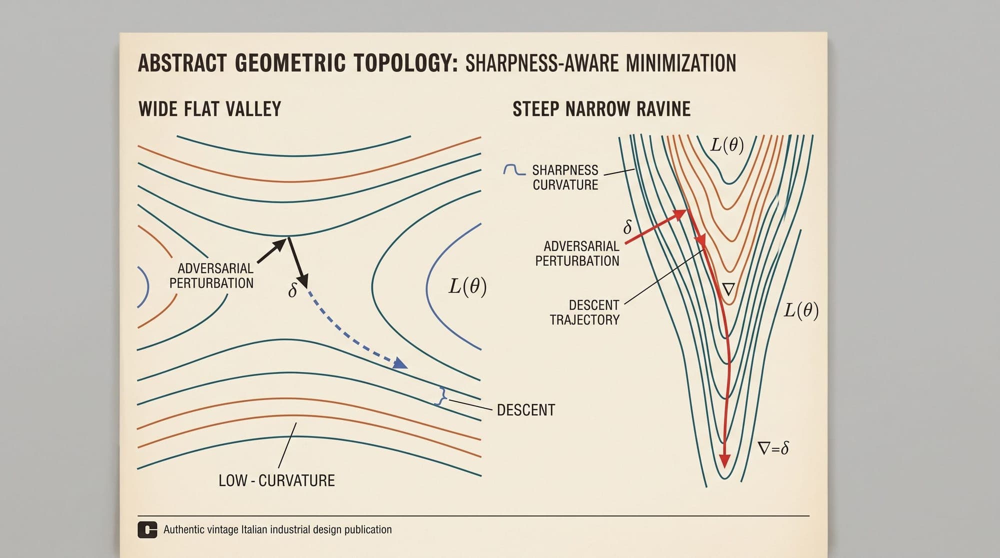
In overparameterized deep neural networks, minimizing empirical training loss is insufficient to guarantee optimal generalization on unseen distributions. Modern deep architectures, including vision models and autoregressive Large Language Models (LLMs), operate in regimes where parameter counts far exceed training token counts, producing highly non-convex loss surfaces populated by infinite global minima. Standard optimization via Stochastic Gradient Descent (SGD) or AdamW often converges to sharp, narrow valleys in the parameter space. While these sharp minima exhibit near-zero training loss, minor distribution shifts between training and test sets cause steep error spikes.

Sharpness-Aware Minimization (SAM), introduced by Foret et al. (ICLR 2021), reformulates gradient optimization as a min-max game. Rather than minimizing the loss value at a single point in parameter space, SAM searches for parameters situated within entire neighborhoods of uniformly low loss. By computing an adversarial weight perturbation that maximizes loss within a bounded Euclidean ball and updating weights based on the gradient at that perturbed point, SAM explicitly penalizes loss landscape sharpness. Applied to language models by Bahri, Mobahi, and Tay (ACL 2022), SAM substantially improves generalization across pre-training and downstream fine-tuning.

1. The Geometry of Generalization: Flat vs. Sharp Minima

The link between loss landscape geometry and generalization was formalized empirically by Keskar et al. (ICLR 2017), who observed that large-batch training tends to land in sharp minima with poor out-of-sample performance, whereas small-batch training benefits from stochastic noise that pushes parameters toward flatter basins.

Mathematically, the local geometry of the empirical loss $L_S(\mathbf{w})$ around a local minimum $\mathbf{w}^*$ is governed by its Taylor expansion:

$$L_S(\mathbf{w}^* + \boldsymbol{\delta}) \approx L_S(\mathbf{w}^<em>) + \nabla L_S(\mathbf{w}^</em>)^T \boldsymbol{\delta} + \frac{1}{2} \boldsymbol{\delta}^T \nabla^2 L_S(\mathbf{w}^*) \boldsymbol{\delta}$$

At a local minimum, the first-order gradient $\nabla L_S(\mathbf{w}^)$ vanishes. The curvature is therefore determined entirely by the Hessian matrix $\mathbf{H} = \nabla^2 L_S(\mathbf{w}^)$:

• Sharp Minima: Characterized by large eigenvalues $\lambda_{\max}(\mathbf{H})$ and high spectral trace $\operatorname{Tr}(\mathbf{H})$. A small parameter shift $\boldsymbol{\delta}$ induced by test set distribution divergence results in a quadratic explosion of the loss $\frac{1}{2} \boldsymbol{\delta}^T \mathbf{H} \boldsymbol{\delta}$.
• Flat Minima: Characterized by small spectral norm $\|\mathbf{H}\|_2$ and low trace. Even if the evaluation distribution slightly shifts the optimal parameters, the loss remains stable within the wide basin.

2. PAC-Bayesian Generalization Bounds and the SAM Objective

Foret et al. grounded SAM in PAC-Bayesian generalization bounds. For any parameter distribution $\mathcal{Q}$ and prior $\mathcal{P}$, the expected population risk $L_{\mathcal{D}}(\mathbf{w})$ is bounded with probability $1 - \delta$ over the training set $S \sim \mathcal{D}^n$ by:

$$\mathbb{E}_{\mathbf{u} \sim \mathcal{N}(0, \sigma^2 \mathbf{I})}[L_{\mathcal{D}}(\mathbf{w} + \mathbf{u})] \le \max_{\|\boldsymbol{\epsilon}\|_2 \le \rho} L_S(\mathbf{w} + \boldsymbol{\epsilon}) + h\left(\frac{\|\mathbf{w}\|_2^2}{\rho^2}\right)$$

where $\rho > 0$ is the perturbation radius and $h(\cdot)$ is a strictly monotonic regularization function.

To minimize this upper bound, SAM optimizes the perturbed loss objective:

$$\min_{\mathbf{w}} L_S^{\text{SAM}}(\mathbf{w}) \triangleq \min_{\mathbf{w}} \left[ \max_{\|\boldsymbol{\epsilon}\|_2 \le \rho} L_S(\mathbf{w} + \boldsymbol{\epsilon}) \right]$$

This objective decomposes directly into standard empirical risk plus a sharpness penalty term:

$$L_S^{\text{SAM}}(\mathbf{w}) = L_S(\mathbf{w}) + \underbrace{\left[ \max_{\|\boldsymbol{\epsilon}\|_2 \le \rho} L_S(\mathbf{w} + \boldsymbol{\epsilon}) - L_S(\mathbf{w}) \right]}_{\text{Sharpness}_\rho(\mathbf{w})}$$

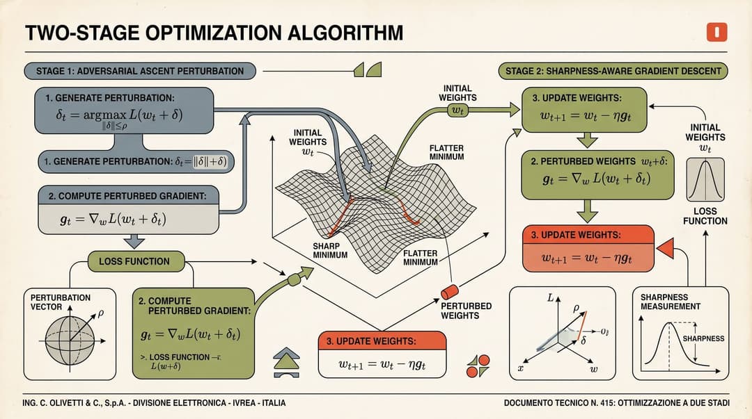
3. The SAM Algorithm: Dual-Phase Min-Max Step

Directly computing the exact inner maximization $\max_{\|\boldsymbol{\epsilon}\|_2 \le \rho} L_S(\mathbf{w} + \boldsymbol{\epsilon})$ at every step is intractable. SAM solves this via a first-order Taylor approximation around $\mathbf{w}$:

$$L_S(\mathbf{w} + \boldsymbol{\epsilon}) \approx L_S(\mathbf{w}) + \boldsymbol{\epsilon}^T \nabla_{\mathbf{w}} L_S(\mathbf{w})$$

Subject to the norm constraint $\|\boldsymbol{\epsilon}\|_2 \le \rho$, the linear program achieves its maximum when $\boldsymbol{\epsilon}$ aligns parallel to the gradient vector $\nabla_{\mathbf{w}} L_S(\mathbf{w})$:

$$\boldsymbol{\epsilon}^*(\mathbf{w}) = \arg\max_{\|\boldsymbol{\epsilon}\|_2 \le \rho} \left\{ \boldsymbol{\epsilon}^T \nabla_{\mathbf{w}} L_S(\mathbf{w}) \right\} = \rho \frac{\nabla_{\mathbf{w}} L_S(\mathbf{w})}{\|\nabla_{\mathbf{w}} L_S(\mathbf{w})\|_2}$$

Once the adversarial perturbation $\boldsymbol{\epsilon}^*(\mathbf{w})$ is determined, SAM updates the original weights $\mathbf{w}$ using the gradient evaluated at the perturbed position:

$$\mathbf{g}_{\text{SAM}} = \nabla_{\mathbf{w}} L_S(\mathbf{w} + \boldsymbol{\epsilon}^*(\mathbf{w}))$$

$$\mathbf{w}_{t+1} = \mathbf{w}_t - \eta \left[ \mathbf{g}_{\text{SAM}} + \lambda \mathbf{w}_t \right]$$

where $\eta$ is the learning rate and $\lambda$ is the weight decay coefficient.

Sharpness-Aware Minimization Step Execution:
1. Sample mini-batch B = {(x_i, y_i)}_{i=1}^m
2. Compute base gradient: g = (1/m) * sum(grad_w L(x_i, y_i; w_t))
3. Calculate worst-case perturbation: epsilon = rho * (g / ||g||_2)
4. Compute sharpness-penalized gradient: g_sam = (1/m) * sum(grad_w L(x_i, y_i; w_t + epsilon))
5. Apply weight update to base parameters: w_{t+1} = Optimizer_Step(w_t, g_sam)

4. Scale Invariance and Adaptive SAM (ASAM)

A theoretical limitation of standard SAM is its lack of scale invariance. In architectures containing Layer Normalization or RMSNorm, multiplying a layer's weight tensor $\mathbf{W}_l$ by a constant $\alpha > 0$ and dividing the subsequent layer by $\alpha$ leaves the model's forward function identical. However, the Euclidean radius $\|\boldsymbol{\epsilon}\|_2 \le \rho$ imposes an isotropic sphere that treats all parameters equally regardless of their magnitude.

To eliminate this artifact, Kwon et al. (ICML 2021) proposed Adaptive SAM (ASAM). ASAM defines the perturbation constraint in a parameter-scaled norm:

$$\boldsymbol{\epsilon}^*_i(\mathbf{w}) = \rho \frac{|w_i| g_i}{\| |\mathbf{w}| \odot \mathbf{g} \|_2}$$

where $\odot$ denotes element-wise multiplication. ASAM scales the perturbation proportionally to the absolute magnitude of each individual weight, ensuring that layers with large parameter values receive proportionately larger perturbations, preserving scale invariance across Transformer blocks.

5. SAM in Transformers and Large Language Models

In natural language processing, Transformer architectures exhibit distinct loss landscape properties compared to convolutional networks. Bahri et al. (ACL 2022) conducted extensive empirical evaluations applying SAM and ASAM to T5, BERT, and RoBERTa across pre-training and downstream GLUE/SuperGLUE benchmarks.

Their findings revealed critical operational dynamics:

• Pre-Training Loss vs. Downstream Generalization: While SAM models often show slightly higher training loss during early pre-training epochs due to the adversarial perturbation penalty, they achieve consistently lower validation perplexity and higher zero-shot/few-shot downstream transfer scores.
• Perturbation Radius Tuning: For language models trained with AdamW, optimal perturbation radii $\rho$ are typically an order of magnitude smaller than those used in vision models (for instance, $\rho \in [0.01, 0.05]$ for Transformers compared to $\rho \in [0.05, 0.20]$ for ResNets).
• Robustness to Spurious Correlations: SAM acts as an implicit regularizer against memorization, preventing attention heads from overfitting to high-frequency token co-occurrences.

6. Computational Overhead and Acceleration Techniques

The principal drawback of standard SAM is its computational cost: evaluating both $\nabla L_S(\mathbf{w})$ and $\nabla L_S(\mathbf{w} + \boldsymbol{\epsilon})$ requires two sequential forward-backward passes per optimization step, effectively halving training throughput (100% compute overhead).

To mitigate this bottleneck, several accelerated variants have been developed:

• LookSAM (Du et al., ICML 2022): Computes the full adversarial perturbation $\boldsymbol{\epsilon}^*$ only once every $k$ steps (typically $k=5$ or $10$). In intermediate steps, LookSAM reuses the gradient direction from the projection step, reducing the compute overhead from 100% down to under 15% with minimal generalization loss.
• Surrogate Gap Minimization / GSAM (Zhuang et al., ICLR 2022): Decomposes the gradient update into two orthogonal vectors: one minimizing the empirical loss and the other minimizing the surrogate gap ($L_S(\mathbf{w} + \boldsymbol{\epsilon}) - L_S(\mathbf{w})$), preventing gradient cancellation and speeding up convergence.
• Micro-Batch SAM in Distributed Sharding: In FSDP and Megatron-LM tensor parallel setups, computing the global gradient norm $\|\mathbf{g}\|_2$ requires an All-Reduce across all ranks before constructing $\boldsymbol{\epsilon}$. Sharded implementations compute layer-local norms to avoid synchronization overhead during the ascent step.

7. Comparative Architectural Trade-Offs

• Standard SGD / AdamW: Operates with 1 forward-backward pass per step (1x overhead). Relies solely on stochastic batch noise for implicit regularization without explicit bounds on Hessian eigenvalues. Lacks scale invariance.
• Weight Decay ($L_2$ Regularization): Adds parameter norm penalty with 1x overhead. Provides weak indirect shrinkage without directly controlling loss surface curvature.
• Stochastic Weight Averaging (SWA): Averages checkpoint weights along the trajectory with periodic evaluation overhead. Traverses toward the center of flat loss basins without modifying inner gradient steps. Scale invariant.
• Sharpness-Aware Minimization (SAM): Employs adversarial minimax weight perturbation with 2x overhead. Explicitly bounds the maximum eigenvalue $\lambda_{\max}(\mathbf{H})$ of the loss Hessian. Lacks scale invariance under layer scaling.
• Adaptive SAM (ASAM): Uses weight-magnitude-scaled perturbations with 2x overhead. Normalizes curvature bounds across layers, restoring scale invariance in normalized Transformer blocks.
• LookSAM: Amortizes minimax perturbations every $k$ iterations, reducing compute overhead to approximately 1.15x while maintaining curvature regularization.

Sources

• Sharpness-Aware Minimization for Efficiently Improving Generalization (Foret et al., ICLR 2021)
• Sharpness-Aware Minimization Improves Language Model Generalization (Bahri, Mobahi, Tay, ACL 2022)
• On Large-Batch Training for Deep Learning: Generalization Gap and Sharp Minima (Keskar et al., ICLR 2017)
• ASAM: Adaptive Sharpness-Aware Minimization for Scale-Invariant Learning of Deep Neural Networks (Kwon et al., ICML 2021)
• Surrogate Gap Minimization Improves Sharpness-Aware Minimization (Zhuang et al., ICLR 2022)
• Sharpness-Aware Minimization for Efficiently Improving Generalization: Fast SAM and LookSAM (Du et al., ICML 2022)