Self-Play Fine-Tuning (SPIN): Mathematical Foundations, Two-Player Minimax Games, and Iterative Distribution Alignment

Supervised Fine-Tuning (SFT) has served as the baseline method for converting pre-trained foundation models into instruction-following assistants. By training on curated prompt-response pairs $(x, y)$ via Maximum Likelihood Estimation (MLE), SFT aligns the model's next-token distributions with human demonstrations.

However, standard SFT exhibits fundamental theoretical limitations. Maximum likelihood training optimizes forward Kullback-Leibler (KL) divergence, forcing the model into mode-covering behavior where it assigns non-zero probability mass across diffuse human phrasing rather than sharpening around optimal responses. Furthermore, SFT suffers from exposure bias: during inference, autoregressive generation compounds errors when the model drifts from the training distribution, as it was never penalized on its own self-generated mistakes.

To surpass the SFT plateau, standard alignment pipelines introduce Reinforcement Learning from Human Feedback (RLHF) or Direct Preference Optimization (DPO). Both paradigms require expensive external annotations, such as pairwise human preference datasets $(x, y_w, y_l)$ or external AI reward models.

Self-Play Fine-Tuning (SPIN), introduced by Chen et al. (2024) at UCLA, provides a game-theoretic alternative. SPIN enables a language model to improve iteratively by playing a two-player zero-sum game against previous versions of itself using only the original SFT dataset, eliminating the need for additional human preference labels or reward models.

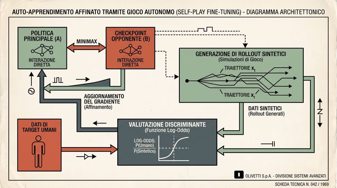
The Mathematical Framework: Two-Player Minimax Game

SPIN casts post-training alignment as a two-player game between an active policy $p_\theta$ (the main player) and a fixed reference policy $p_{\theta_t}$ from the previous iteration (the opponent player).

Let $q(x)$ denote the prompt distribution and $p_{\text{data}}(y|x)$ denote the ground-truth target data distribution from the SFT dataset. The objective of the main player is to maximize a value function that discriminates human demonstrations from synthetic rollouts generated by the opponent:

$$\max_{p} \min_{p'} \mathbb{E}_{x \sim q(\cdot)} \left[ \mathbb{E}_{y \sim p_{\text{data}}(\cdot|x)} [f(x, y)] - \mathbb{E}_{y' \sim p'(\cdot|x)} [f(x, y')] \right]$$

where $f(x, y)$ is a discriminator function measuring the likelihood that response $y$ was drawn from $p_{\text{data}}$ rather than the opponent $p'$.

KL-Constrained Value Optimization

To prevent policy collapse and ensure stable gradient updates, SPIN constrains the optimization of the main player $p$ relative to the opponent policy $p_{\theta_t}$ using KL divergence:

$$\max_{p} \mathbb{E}_{x \sim q(x)} \left[ \mathbb{E}_{y \sim p_{\text{data}}(\cdot|x)} [f(x, y)] - \mathbb{E}_{y' \sim p_{\theta_t}(\cdot|x)} [f(x, y')] \right] - \lambda \mathbb{D}_{\text{KL}}(p(\cdot|x) \parallel p_{\theta_t}(\cdot|x))$$

where $\lambda > 0$ is a regularization parameter controlling the penalty for deviating from the reference policy $p_{\theta_t}$.

By solving the Karush-Kuhn-Tucker (KKT) conditions for the constrained optimization problem over the probability simplex $\sum_y p(y|x) = 1$, the optimal closed-form policy $p^*(y|x)$ satisfies:

$$p^*(y|x) = \frac{p_{\theta_t}(y|x) \exp\left( \frac{1}{\lambda} f(x, y) \right)}{Z(x)}$$

where $Z(x) = \sum_y p_{\theta_t}(y|x) \exp\left( \frac{1}{\lambda} f(x, y) \right)$ is the partition function.

Inverting this relationship expresses the discriminator function $f(x, y)$ directly in terms of the log-ratio between the active policy and the opponent policy:

$$f(x, y) = \lambda \log \frac{p(y|x)}{p_{\theta_t}(y|x)} + \lambda \log Z(x)$$

The Closed-Form SPIN Loss Function

Substituting the reparameterized discriminator back into the minimax game and applying a logistic loss surrogate $\ell(u) = \log(1 + e^{-u})$ eliminates the intractable partition function $Z(x)$. This yields the closed-form SPIN objective for iteration $t$:

$$\mathcal{L}_{\text{SPIN}}(\theta, \theta_t) = \mathbb{E}_{x \sim q(\cdot), y \sim p_{\text{data}}(\cdot|x), y' \sim p_{\theta_t}(\cdot|x)} \left[ \ell \left( \lambda \log \frac{p_\theta(y|x)}{p_{\theta_t}(y|x)} - \lambda \log \frac{p_\theta(y'|x)}{p_{\theta_t}(y'|x)} \right) \right]$$

Expanding the logistic function gives the practical training loss:

$$\mathcal{L}_{\text{SPIN}}(\theta, \theta_t) = \mathbb{E}_{(x, y, y')} \left[ \log \left( 1 + \exp \left( -\lambda \left( \log \frac{p_\theta(y|x)}{p_{\theta_t}(y|x)} - \log \frac{p_\theta(y'|x)}{p_{\theta_t}(y'|x)} \right) \right) \right) \right]$$

During gradient descent, the parameter update increases the log-likelihood of target demonstration $y$ under $p_\theta$ while penalizing the log-likelihood of the self-generated synthetic response $y'$, scaled by their relative odds against the previous checkpoint $p_{\theta_t}$.

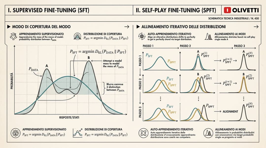
Theoretical Guarantees and Nash Equilibrium

The central theoretical property of SPIN is that the global Nash equilibrium of the two-player game is achieved if and only if the model's policy matches the target data distribution.

Global Convergence Theorem

Let $\mathcal{P}$ denote the space of all valid conditional probability distributions over responses given prompts. If the function class parameterized by $\theta$ has sufficient capacity, the two-player optimization problem satisfies:

$$p_\theta(y|x) = p_{\text{data}}(y|x) \quad \forall x \in \text{supp}(q)$$

Proof Sketch:

1. At iteration $t$, assume the opponent has converged to the target distribution, $p_{\theta_t}(y|x) = p_{\text{data}}(y|x)$.
2. The argument inside the logistic loss function becomes:

$$\Delta(x, y, y') = \lambda \log \frac{p_\theta(y|x)}{p_{\text{data}}(y|x)} - \lambda \log \frac{p_\theta(y'|x)}{p_{\text{data}}(y'|x)}$$

1. When $p_\theta(y|x) = p_{\text{data}}(y|x)$, the log-ratio $\log \frac{p_\theta(y|x)}{p_{\text{data}}(y|x)} = 0$ for all $y$, leading to $\Delta(x, y, y') = 0$.
2. The gradient of the loss with respect to parameters $\theta$ vanishes:

$$\nabla_\theta \mathcal{L}_{\text{SPIN}}(\theta, \theta_t) \Big|_{p_\theta = p_{\theta_t} = p_{\text{data}}} = 0$$

1. Because $\ell(u)$ is strictly convex and monotonically decreasing, any distribution $p_\theta \neq p_{\text{data}}$ yields a strictly positive expected gradient pulling $p_\theta$ toward $p_{\text{data}}$. Thus, $p_\theta = p_{\text{data}}$ is the unique stationary point and global Nash equilibrium of the dynamical system.

Why SPIN Avoids GAN Instabilities

Traditional Generative Adversarial Networks (GANs) parameterized with separate generator and discriminator networks frequently suffer from mode collapse, vanishing gradients, and rotational limit cycles. SPIN avoids these failure modes through two architectural properties:

1. Implicit Discriminator Parameterization: SPIN does not train an auxiliary neural network discriminator. The discriminator is derived analytically from the language model's own token-level logits, ensuring the discriminator and generator evolve in lockstep.
2. Local KL Anchoring: Each iteration anchors the policy to the previous checkpoint $p_{\theta_t}$ rather than an unconstrained search space, preventing destructive policy drift.

Iterative Multi-Stage Training Pipeline

SPIN operates as an iterative multi-round algorithm. Starting from an initial SFT checkpoint $\theta_0$, each round consists of two sequential phases:

Algorithm: Self-Play Fine-Tuning (SPIN)
Input: SFT dataset D = {(x_i, y_i)}_{i=1}^N, Initial SFT model theta_0, Regularizer lambda, Iterations T
Output: Final aligned model theta_T

For t = 0 to T - 1 do:
    1. Generation Phase:
       For each prompt x_i in D:
           Sample synthetic response y'_i ~ p_{theta_t}(. | x_i)
       Construct synthetic dataset D_t = {(x_i, y_i, y'_i)}_{i=1}^N
    
    2. Alignment Phase:
       Initialize theta_{t+1} <- theta_t
       Train theta_{t+1} by minimizing L_SPIN(theta, theta_t) over D_t
       Update opponent checkpoint: theta_t <- theta_{t+1}
End For

Dynamic Hard Negative Mining

In iteration 0, the baseline model $\theta_0$ generates responses $y'$ that contain obvious hallucinations, structural disorganization, and reasoning errors. Distinguishing real data $y$ from $y'$ at iteration 0 is relatively easy.

As the model advances to iterations 1 and 2, $p_{\theta_t}$ produces high-fluency responses that closely mirror human structure. The synthetic rollouts $y'$ become fine-grained hard negatives. Minimizing $\mathcal{L}_{\text{SPIN}}$ in later iterations forces the model to eliminate subtle logical inconsistencies and stylistic divergence that simple cross-entropy SFT cannot penalize.

Saturation Dynamics and Diminishing Returns

Empirical evaluations across open benchmarks indicate that SPIN yields substantial performance gains during iterations 1 and 2, with gains plateauing around iterations 3 and 4:

• Iteration 0 to 1: Major step-function improvement across reasoning (GSM8k), truthfulness (TruthfulQA), and instruction following (MT-Bench).
• Iteration 1 to 2: Incremental refinement in factual precision and formatting compliance.
• Iteration 3+: Performance saturates as synthetic responses $y'$ approach the empirical support of $p_{\text{data}}$, while fixed prompt sets $q(x)$ bound the total novel signal extractable from the dataset.

Comparative Analysis: SFT, DPO, STaR, and SPIN

Understanding where SPIN fits within modern post-training workflows requires comparing its optimization mechanics against related alignment techniques:

• Supervised Fine-Tuning (SFT):
• Loss Formulation: Cross-entropy MLE: $\mathcal{L}_{\text{SFT}} = -\mathbb{E}_{(x, y)} [\log p_\theta(y|x)]$.
• Data Required: Demonstration pairs $(x, y)$.
• Mechanism: Mode covering; maximizes unconditional likelihood on target tokens without negative contrast.
• Direct Preference Optimization (DPO):
• Loss Formulation: Pairwise Bradley-Terry preference loss over winner/loser pairs: $\mathcal{L}_{\text{DPO}} = -\mathbb{E}_{(x, y_w, y_l)} [\log \sigma(\beta \log \frac{p_\theta(y_w|x)}{p_{\text{ref}}(y_w|x)} - \beta \log \frac{p_\theta(y_l|x)}{p_{\text{ref}}(y_l|x)})]$.
• Data Required: Preference pairs $(x, y_w, y_l)$ annotated by humans or frontier judge models.
• Mechanism: Directly aligns policy to external preference rankings using fixed offline reference $p_{\text{ref}}$.
• Self-Taught Reasoner (STaR):
• Loss Formulation: Rejection sampling + SFT: $\mathcal{L}_{\text{STaR}} = -\mathbb{E}_{(x, y')} [\mathbb{I}(R(y') = 1) \log p_\theta(y'|x)]$.
• Data Required: Prompts with verifiable ground-truth reward functions $R(y') \in \{0, 1\}$ (e.g., math or unit tests).
• Mechanism: Filters model rollouts through deterministic verifiers and retrains on successful rationales.
• Self-Play Fine-Tuning (SPIN):
• Loss Formulation: Iterative minimax logistic loss: $\mathcal{L}_{\text{SPIN}}(\theta, \theta_t)$.
• Data Required: SFT dataset $(x, y)$ only; no preference annotations or programmatic verifiers.
• Mechanism: Self-generates negative rollouts $y'$ at each iteration, optimizing relative log-odds against target human demonstrations.

Empirical Results and Implementation Details

In the original evaluations by Chen et al. (2024), SPIN was evaluated on the UltraChat dataset using base Zephyr-7B and Mistral-7B models:

• HuggingFace Open LLM Leaderboard: SPIN improved the average benchmark score of Zephyr-7B-SFT from 58.14 to 63.16 without using external preference data.
• Reasoning and Truthfulness: GSM8k accuracy improved by over 10 percentage points, while TruthfulQA scores rose from 43.8% to 54.2%.
• Multi-Turn Chat (MT-Bench): MT-Bench score improved from 5.94 (SFT baseline) to 6.78 at iteration 1, rivaling models trained with DPO on 62k labeled pairwise preference samples (UltraFeedback).

Hyperparameter Settings

Practical implementations of SPIN (e.g., in Hugging Face TRL and verl) rely on the following tuning guidelines:

1. Regularization Parameter ($\lambda$ / $\beta$): $\lambda$ is equivalent to $1/\beta$ in DPO literature. Common configurations set $\lambda = 10.0$ (corresponding to $\beta = 0.1$). Larger $\lambda$ values enforce tighter adherence to the reference checkpoint $\theta_t$, preventing policy entropy collapse.
2. Generation Temperature: During the rollout generation phase, sampling temperatures between $T = 0.7$ and $T = 1.0$ provide sufficient diversity in negative candidate responses $y'$.
3. Learning Rate Schedules: Typical learning rates range from $5 \times 10^{-7}$ to $1 \times 10^{-6}$ with cosine decay, using DeepSpeed ZeRO-3 or FSDP to manage memory during gradient accumulation.

Sources

• Chen, Z., Deng, Y., Yuan, H., Ji, K., & Gu, Q. (2024). Self-Play Fine-Tuning Converts Weak Language Models to Strong Language Models. International Conference on Machine Learning (ICML 2024).
• Rafailov, R., Sharma, A., Mitchell, E., Ermon, S., Manning, C. D., & Finn, C. (2023). Direct Preference Optimization: Your Language Model Is Secretly a Reward Model. Advances in Neural Information Processing Systems (NeurIPS 2023).
• Zelikman, E., Wu, Y., Mu, J., & Goodman, N. (2022). STaR: Bootstrapping Reasoning With Reasoning. Advances in Neural Information Processing Systems (NeurIPS 2022).
• Tunstall, L., Beeching, E., Lambert, N., Rajani, N., Rasul, K., Belkada, Y., Huang, S., von Werra, L., Fourrier, C., Habib, N., Sarrazin, N., Sanseviero, O., Rush, A. M., & Wolf, T. (2023). Zephyr: Direct Distillation of LM Alignment. arXiv preprint arXiv:2310.16944.