Multi-Head Latent Attention: How Low-Rank KV Compression Scales LLM Serving

Autoregressive transformer inference faces a fundamental hardware constraint during text generation: memory bandwidth saturation. While prefill (processing prompt tokens) is compute-bound and saturates GPU tensor cores, token-by-token generation is memory-bandwidth bound. To generate each subsequent token, the inference engine must load all prior Key and Value vectors from High Bandwidth Memory (HBM) into SRAM.

As sequence lengths reach 32k, 64k, or 128k tokens and batch sizes scale, the Key-Value (KV) cache dominates accelerator memory. Multi-Head Latent Attention (MLA), introduced by DeepSeek in the DeepSeek-V2 technical report and scaled in DeepSeek-V3, redesigns the transformer attention module around low-rank compression. MLA reduces the KV cache memory footprint by up to 93 percent compared to standard Multi-Head Attention while retaining the representational capacity of large multi-head configurations.

The Memory Bottleneck in Transformer Attention

In standard Multi-Head Attention (MHA), an input sequence produces query, key, and value representations across $n_h$ attention heads, each with dimension $d_h$ . For an input hidden state $h_t \in \mathbb{R}^d$ , the projections are:

q_t = W^Q h_t
k_t = W^K h_t
v_t = W^V h_t

During generation, the keys and values for every past token must be retained in memory. For a model with $n_l$ layers, sequence length $L$ , batch size $B$ , and 16-bit precision (2 bytes per float), the KV cache size in bytes is:

KV_Cache_Size = 2 * 2 * n_l * n_h * d_h * L * B

For a 128-head model with head dimension 128, each token across all layers requires storing $2 \times 128 \times 128 = 32,768$ values per layer. On long contexts, this footprint exhausts GPU memory, strictly limiting batch sizes and causing decoding throughput to stall on memory transfers.

Multi-Head Latent Attention Architecture and Key-Value Compression

Prior architectures attempted to mitigate this overhead by reducing head counts:

Multi-Query Attention (MQA) collapses all key and value heads into a single shared KV head ( $n_{kv} = 1$ ). While this cuts cache footprint by $n_h$ , it severely restricts the model capacity to attend to distinct feature subspaces.
Grouped-Query Attention (GQA) partitions query heads into $G$ groups, sharing one KV head per group (e.g., 8 KV heads for 64 or 128 query heads, as used in LLaMA models). GQA provides a middle ground but still enforces a trade-off between cache savings and representational diversity.

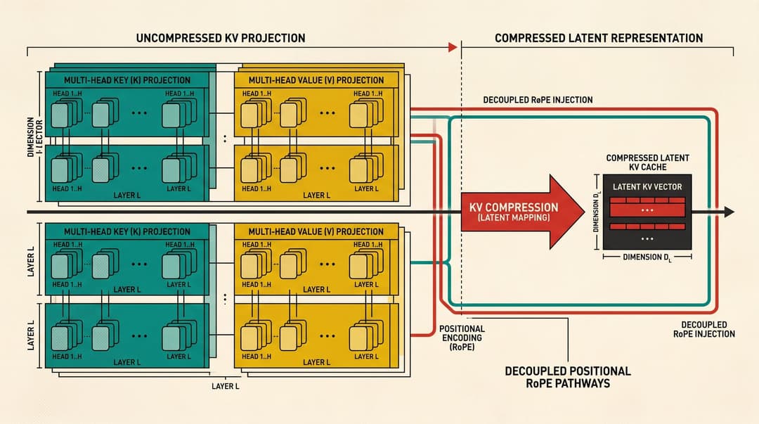
MLA takes an alternative mathematical approach: instead of pruning heads, it compresses the entire key-value space into a low-dimensional latent vector via low-rank matrix decomposition.

Low-Rank Key-Value Joint Compression

Rather than projecting the hidden state $h_t$ into separate high-dimensional keys and values, MLA projects $h_t$ into a compact latent vector $c_t^{KV} \in \mathbb{R}^{d_c}$ using a down-projection matrix $W^{DKV} \in \mathbb{R}^{d_c \times d}$ :

c_t^{KV} = W^{DKV} h_t

Where $d_c \ll n_h d_h$ . The full multi-head content keys and content values are then recovered through up-projection matrices $W^{UK} \in \mathbb{R}^{n_h d_h \times d_c}$ and $W^{UV} \in \mathbb{R}^{n_h d_h \times d_c}$ :

k_{t,i}^C = W_i^{UK} c_t^{KV}
v_{t,i}^C = W_i^{UV} c_t^{KV}

To reduce activation memory during training, MLA also applies low-rank compression to the queries:

c_t^Q = W^{DQ} h_t
q_{t,i}^C = W_i^{UQ} c_t^Q

Where $c_t^Q \in \mathbb{R}^{d_c'}$ and $W^{DQ} \in \mathbb{R}^{d_c' \times d}$ .

The Positional Problem and Decoupled RoPE

Modern transformers rely on Rotary Position Embedding (RoPE) to inject relative positional information by multiplying keys and queries with position-dependent rotation matrices:

q_rotated = RoPE(q, position)
k_rotated = RoPE(k, position)

However, applying RoPE directly to the up-projected keys introduces an algebraic obstacle:

k_{t,i} = RoPE(W_i^{UK} c_t^{KV}, t) = R_t (W_i^{UK} c_t^{KV})

Because the rotation matrix $R_t$ sits between the projection matrix $W_i^{UK}$ and the latent vector $c_t^{KV}$ , the projection matrix cannot be pre-multiplied into the query during inference. Without eliminating this dependency, an inference engine would be forced to decompress and rotate full key vectors for every historical token, discarding the memory bandwidth advantage.

To resolve this, MLA introduces Decoupled RoPE. Rather than applying rotation to the compressed content vectors, the architecture separates content representations from positional representations:

Content Keys and Queries: $k_{t,i}^C$ and $q_{t,i}^C$ carry semantic content without positional rotation.
Positional Keys and Queries: Dedicated low-dimensional vectors $k_t^R \in \mathbb{R}^{d_R}$ and $q_{t,i}^R \in \mathbb{R}^{d_R}$ are generated specifically to carry RoPE rotations:

q_{t,i}^R = RoPE(W_i^{QR} c_t^Q, t)
k_t^R = RoPE(W^{KR} h_t, t)

The positional key $k_t^R$ is shared across all attention heads within a layer, minimizing additional parameters and cache overhead.

During attention computation, the content and positional vectors are concatenated:

q_{t,i} = [q_{t,i}^C; q_{t,i}^R]
k_{j,i} = [k_{j,i}^C; k_j^R]

Because inner products distribute over vector concatenation, the attention score calculation splits into two independent terms:

Score_{t, j, i} = (q_{t,i}^C)^T k_{j,i}^C + (q_{t,i}^R)^T k_j^R

Inference Optimization: Weight Matrix Absorption

The mathematical separation of content and position unlocks weight matrix absorption during autoregressive decoding.

During inference, the system never materializes $k_{j,i}^C$ or $v_{j,i}^C$ in GPU memory. The KV cache stores only two tensors per token per layer:

The compressed latent vector $c_j^{KV} \in \mathbb{R}^{d_c}$
The decoupled RoPE key $k_j^R \in \mathbb{R}^{d_R}$

Query Key Absorption

Using the associativity of matrix multiplication, the dot product between the query and the content key is rewritten:

(q_{t,i}^C)^T k_{j,i}^C = (q_{t,i}^C)^T (W_i^{UK} c_j^{KV}) = ((q_{t,i}^C)^T W_i^{UK}) c_j^{KV}

Instead of multiplying every cached $c_j^{KV}$ by $W_i^{UK}$ , the inference engine multiplies the single active query $q_{t,i}^C$ by $W_i^{UK}$ once at the start of the step:

q_{t,i}^{absorbed} = (q_{t,i}^C)^T W_i^{UK}

The attention logits are then computed directly against the compact cached vectors:

Score_{t, j, i} = q_{t,i}^{absorbed} c_j^{KV} + (q_{t,i}^R)^T k_j^R

Value Output Absorption

A similar transformation applies to the attention values. The attention output for head $i$ is:

o_{t,i} = sum_j ( A_{t, j, i} * v_{j,i}^C ) = sum_j ( A_{t, j, i} * (W_i^{UV} c_j^{KV}) )

Factoring out the linear transformation $W_i^{UV}$ :

o_{t,i} = W_i^{UV} ( sum_j ( A_{t, j, i} * c_j^{KV} ) )

The attention mechanism computes the weighted sum over the low-dimensional latent vectors $c_j^{KV}$ first. The up-projection $W_i^{UV}$ is applied once to the aggregated result, or mathematically fused into the output projection matrix $W^O$ .

Quantitative Comparison and Serving Economics

In DeepSeek-V2 and DeepSeek-V3, the attention parameters are configured as:

Number of heads ( $n_h$ ): 128
Head dimension ( $d_h$ ): 128
Latent KV dimension ( $d_c$ ): 512
Decoupled RoPE key dimension ( $d_R$ ): 64

The per-token cache requirements per layer compare as follows:

Standard Multi-Head Attention (128 heads): Stores $2 \times 128 \times 128 = 32,768$ elements per token.
Grouped-Query Attention (8 KV heads): Stores $2 \times 8 \times 128 = 2,048$ elements per token.
Multi-Head Latent Attention: Stores $d_c + d_R = 512 + 64 = 576$ elements per token.

MLA achieves a 98.2 percent reduction in KV cache size compared to full MHA, and a 71.9 percent reduction compared to standard 8-head GQA. Unlike GQA, which restricts the model to 8 key-value heads, MLA allows the network to maintain 128 distinct query heads and full representational subspace diversity.

This reduction directly translates to serving efficiency:

Higher Concurrency: Systems can pack larger batch sizes into fixed GPU memory budgets without triggering out-of-memory errors.
Long-Context Economics: Operating at 128k context windows requires substantially less HBM allocation, reducing server hardware counts.
Bandwidth Saturation Relief: Decoding speed scales almost inversely with memory transfer volume, yielding higher output token throughput during memory-bound generation phases.

Hardware Trade-offs and Tensor Parallelism

While MLA improves memory bandwidth utilization during decoding, it introduces specific hardware trade-offs:

Slightly Higher Arithmetic Operations: Computing the absorbed projections and decoupled RoPE dot products adds floating-point operations. In memory-bandwidth-bound decoding regimes, this compute overhead is negligible compared to memory savings. During dense prefill (where compute dominates), the low-rank projection behaves similarly to standard linear layers.
Tensor Parallelism Sharding: In standard MHA and GQA, attention heads are partitioned cleanly across Tensor Parallel (TP) ranks (e.g., Megatron-LM style). In MLA, the latent vector $c_t^{KV}$ is shared across all heads. Under basic TP implementations, $c_t^{KV}$ must either be duplicated across all GPUs or communicated via collective operations, requiring specialized inference kernels like FlashMLA for optimized multi-GPU deployments.

Multi-Head Latent Attention illustrates how algorithmic matrix restructuring can circumvent physical memory bandwidth limits in modern generative AI infrastructure.