Maximal Update Parametrization (muP): Mathematical Foundations, Infinite-Width Scaling Limits, and Zero-Shot Hyperparameter Transfer in LLM Pre-Training

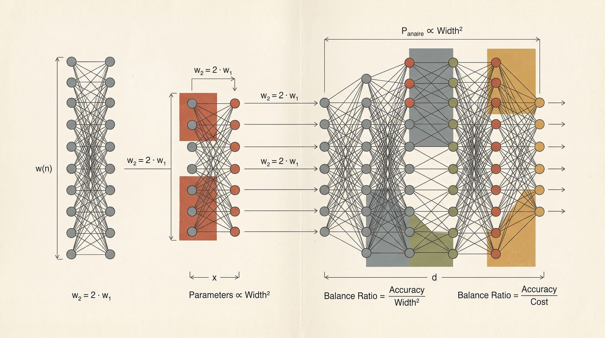
Pre-training large language models requires optimizing sensitive hyperparameters, including learning rate, weight initialization variance, Adam momentum coefficients, and learning rate schedules. In standard neural network implementations, optimal hyperparameters change whenever model dimensions expand. A learning rate tuned on a 125-million parameter model frequently destabilizes or underperforms when applied directly to a 13-billion or 70-billion parameter architecture.

Because grid-searching hyperparameters directly on multi-billion parameter clusters is economically prohibitive, engineering teams historically relied on manual heuristics, trial runs, or conservative learning rates that sacrifice loss convergence.

Maximal Update Parametrization (abbreviated as muP or $\mu$P), introduced by Greg Yang and collaborators at Microsoft Research through the Tensor Programs framework, provides a mathematically rigorous parameterization where optimal hyperparameters remain invariant across model widths. Under muP, practitioners can optimize hyperparameters on a small, single-GPU proxy model and transfer those exact values zero-shot to arbitrarily wide production models.

The Mathematical Breakdown of Standard Parametrization

In the Standard Parametrization (SP) used by default in frameworks such as PyTorch, neural network weights are typically initialized according to Xavier/Glorot or Kaiming initialization schemes, where hidden layer weights $W \in \mathbb{R}^{d \times d}$ have variance scaling as $\Theta(1/d)$.

While standard initialization ensures that the variance of forward activations remains roughly $\Theta(1)$ at initialization (step 0), it fails to preserve consistent representation dynamics once gradient updates begin.

Consider a linear layer $h = W x$, where $x \in \mathbb{R}^d$ and $W \in \mathbb{R}^{d \times d}$. During a step of gradient descent with learning rate $\eta$:

$$\Delta W = -\eta \nabla_W L = -\eta (\delta x^\top)$$

where $\delta = \nabla_h L \in \mathbb{R}^d$. The induced change in hidden representations $\Delta h$ after one update step is:

$$\Delta h = (\Delta W) x = -\eta (\delta x^\top) x = -\eta \delta (x^\top x)$$

In standard parametrization, as width $d \to \infty$:

• The inner product $x^\top x = \sum_{i=1}^d x_i^2$ scales proportionally to the width $d$, or $\Theta(d)$.
• Consequently, the representation update $\Delta h$ scales as $\Theta(\eta \cdot d)$.

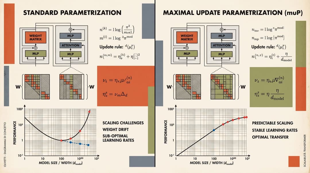
If the global learning rate $\eta$ is held constant as width $d$ grows, the representation update per step explodes at rate $\Theta(d)$. Conversely, if $\eta$ is shrunk to $\Theta(1/d)$ to stabilize feature updates, the network transitions into the "Neural Tangent Kernel (NTK) regime" (also called the lazy training regime), where network weights barely move from initialization and internal representations fail to adaptively extract rich features from the data.

The muP Formalism: Preserving Maximal Feature Learning

Tensor Programs theory proves that muP is the unique parameterization that simultaneously satisfies two constraints in the infinite-width limit ($d \to \infty$):

1. Activations and pre-activations remain bounded at $\Theta(1)$ throughout training.
2. Representation updates $\Delta h$ at every layer remain non-trivial at $\Theta(1)$, preserving maximal feature learning.

To enforce these conditions across all layer types, muP derives specific scaling rules for parameter initialization variance, weight multipliers, and optimizer-specific learning rates based on layer fan-in and fan-out dimensions.

1. Input and Embedding Layers ($d_{in} \to d$)

• Input dimensions (such as vocabulary size or input feature counts) remain fixed while hidden dimension $d$ scales.
• Weight initialization: Variance is set to $\Theta(1)$.
• Learning rate scaling: Global base learning rate $\eta_{base}$ is applied without width discounting, scaling as $\Theta(1)$.

2. Hidden Weight Matrices ($d \to d$)

• Both input and output dimensions grow with model width $d$.
• Weight initialization: Variance is scaled as $\Theta(1/d)$.
• Learning rate scaling: For standard optimizers like Adam and AdamW, the coordinate updates are normalized by coordinate variance. To ensure $\Delta W$ produces $\Delta h = \Theta(1)$, the layer learning rate must scale inversely with width:

$$\eta_{hidden} = \eta_{base} \cdot \frac{d_{base}}{d}$$

where $d_{base}$ is the hidden dimension of the small proxy model and $d$ is the target model width.

3. Readout / Output Projection Layers ($d \to d_{out}$)

• The readout projection maps hidden representations $d$ back to a fixed target space $d_{out}$ (such as vocabulary logits).
• Weight initialization: Variance is scaled as $\Theta(1/d^2)$ or explicitly initialized to zero.
• Output logit multiplier: Logits are scaled by an explicit multiplier factor:

$$\alpha_{output} = \frac{d_{base}}{d}$$

• Learning rate scaling: Scaled as $\Theta(1/d)$ or parameterized via the output multiplier.

Transformer Attention Scaling: Correcting the Softmax Denominator

Standard Transformer architectures calculate scaled dot-product attention using a scaling factor of $1/\sqrt{d_{head}}$:

$$\text{Attention}(Q, K, V) = \text{softmax}\left(\frac{Q K^\top}{\sqrt{d_{head}}}\right) V$$

The original $1/\sqrt{d_{head}}$ factor was chosen assuming that query vector $q$ and key vector $k$ are independent, zero-mean random variables at initialization, meaning their inner product variance grows as $\Theta(\sqrt{d_{head}})$ by the Central Limit Theorem.

However, during optimization, queries and keys become correlated as attention heads learn semantic associations. When $q$ and $k$ align, the inner product $q^\top k = \sum_{i=1}^{d_{head}} q_i k_i$ scales linearly with dimension $\Theta(d_{head})$ by the Law of Large Numbers.

Under muP, attention logits are scaled by $1/d_{head}$ (or an equivalent attention multiplier $\alpha_{attn} = d_{base\_head} / d_{head}$) rather than $1/\sqrt{d_{head}}$. This adjustment prevents attention entropy from collapsing into one-hot delta distributions as model width and head dimension scale up.

The Coordinate Check Diagnostic

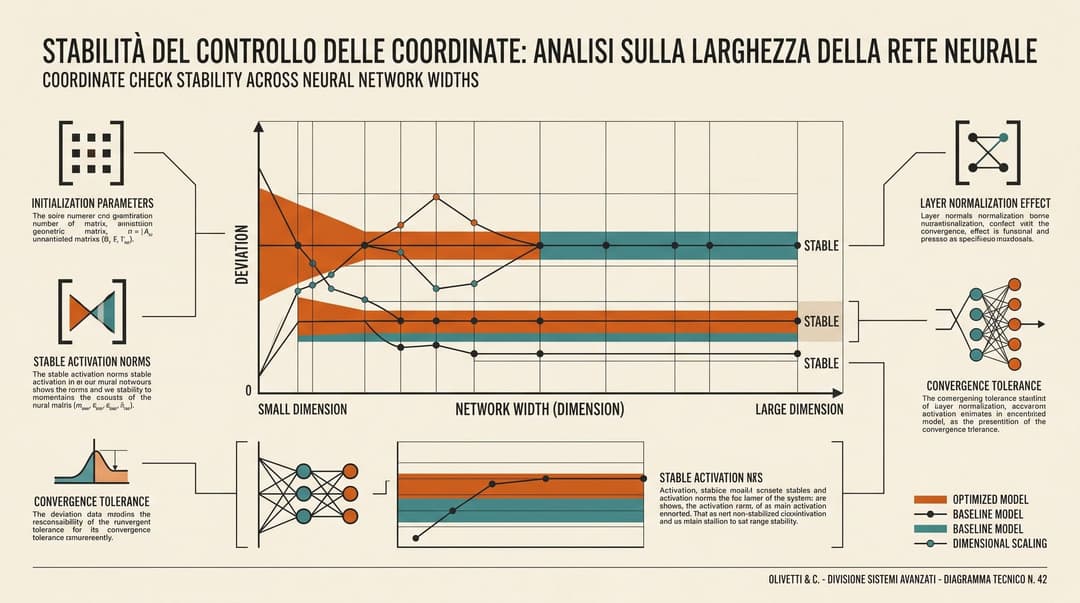
Before committing massive compute budgets to large-scale training runs, practitioners verify their muP implementation using a coordinate check (coord_check).

A coordinate check tracks the mean absolute update of layer activations over initial training steps across models of exponentially increasing widths (for example, $d \in \{128, 256, 512, 1024, 2048, 4096\}$):

1. Failure Mode (Standard Parametrization): The mean activation update norm $\|\Delta h\|$ forms upward-sloping curves proportional to width $d$, demonstrating parameter instability.
2. Success Mode (muP): Activation update norms across all layers collapse into flat, overlapping horizontal lines, confirming that update magnitudes are scale-invariant at $\Theta(1)$.

Zero-Shot Hyperparameter Transfer (muTransfer) in Production

The primary engineering deliverable of muP is muTransfer: the ability to perform rigorous hyperparameter sweeps on tiny models and transfer the optimal configuration directly to frontier-scale foundation models.

The production workflow proceeds in four distinct stages:

1. Proxy Architecture Selection: Construct a base model with identical depth, vocabulary, and activation functions, but with narrow width (for example, a 13-million or 110-million parameter proxy with $d_{base} = 256$ or $512$).
2. Comprehensive Grid Sweeps: Run automated hyperparameter searches over learning rate, Adam $\beta_1$ and $\beta_2$, weight decay, and learning rate warmup ratios on the proxy model using standard compute instances.
3. Parameter Rescaling: Apply the muP width scaling multipliers to hidden layers, readout projections, and attention blocks for the target architecture (such as a 7-billion, 13-billion, or 70-billion parameter model).
4. Direct Pre-Training Launch: Initialize the full-scale model using the transferred optimal hyperparameters without conducting exploratory tuning runs at scale.

Empirical validations by Microsoft Research and Cerebras Systems demonstrated that models trained with muTransfer achieve lower validation perplexity than standard parameterization baselines while eliminating the multi-million dollar overhead of large-scale hyperparameter trial runs.

Sources

• Tensor Programs V: Tuning Large Neural Networks via Zero-Shot Hyperparameter Transfer (Yang et al., Microsoft Research / NeurIPS 2021)
• Tensor Programs IV: Feature Learning in Infinite-Width Neural Networks (Yang & Hu, ICML 2021)
• Maximal Update Parametrization (muP) GitHub Repository (Microsoft)
• The Practitioner's Guide to the Maximal Update Parameterization (Cerebras Systems)
• Cerebras-GPT: A Family of Open, Compute-Efficient Language Models (Dey et al., Cerebras Systems / arXiv 2023)