Compound AI Systems in Production: Architecture, Co-Optimization, and Error Cascades

For the first two years following the release of GPT-4, enterprise AI development focused almost exclusively on model-centric scaling: upgrading to larger parameter checkpoints, expanding prompt context windows, and tuning system prompts. However, production deployments quickly revealed a fundamental constraint: single, monolithic foundation models exhibit diminishing returns on high-complexity, multi-step tasks.

According to research from the Berkeley AI Research (BAIR) Lab, state-of-the-art results across code synthesis, mathematical reasoning, and enterprise automation are increasingly driven by Compound AI Systems: systems that tackle complex tasks using multiple interacting components, including specialized models, external retrievers, sandboxed execution runtimes, and symbolic verifiers.

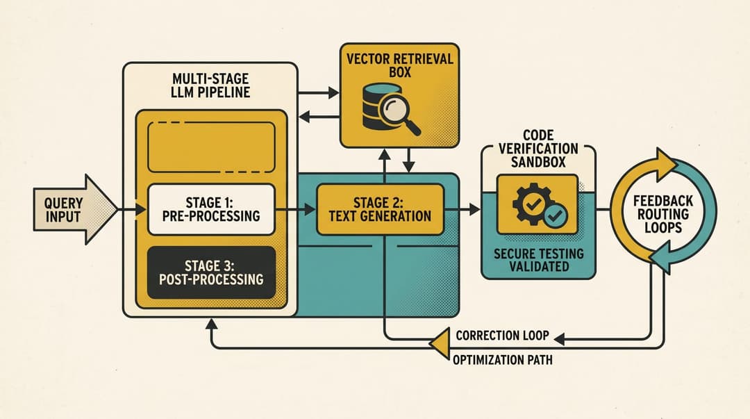
Engineering compound AI architectures introduces distinct systems challenges that do not exist in single-model prompting. Building reliable multi-component AI pipelines requires understanding architectural topologies, compounding failure probabilities, non-differentiable co-optimization, and tight latency budgets.

1. The Architectural Topologies of Compound AI Systems

Unlike a monolithic model that accepts a single prompt and emits a single completion, a compound AI system structures inference across discrete, modular stages. Industry production systems generally follow four primary topological patterns:

A. Dynamic Cascades and Speculative Routing

In high-throughput enterprise workloads, sending every query to a frontier model incurs prohibitive latency and cost. Cascade architectures evaluate queries hierarchically:

1. A lightweight classifier or small language model (1B to 8B parameters) evaluates query complexity and produces an initial draft or classification.
2. An automated confidence scorer determines whether the draft satisfies task criteria.
3. If uncertainty exceeds a predefined threshold, the query escalates to a larger frontier model.

This pattern, formalized by frameworks like FrugalGPT, reduces inference expenditure by up to 70% to 90% while matching or exceeding the accuracy of unrouted frontier models on standard benchmarks.

B. Neuro-Symbolic Hybrid Loops

Pure neural models struggle with strict arithmetic, formal logic, and syntax enforcement. Neuro-symbolic compound systems pair the inductive pattern-matching capabilities of transformers with deterministic engines.

• Google DeepMind's AlphaGeometry demonstrates this pattern by combining a fine-tuned LLM with a symbolic geometry deduction engine. When the symbolic engine hits a proof impasse, the LLM generates a geometric auxiliary construction. The symbolic solver then resumes deterministic deductions, achieving Olympiad-level performance without hallucinations in the formal proof.

C. Mass Sampling, Execution, and Clustering

Rather than relying on greedy decoding or single-trajectory sampling, systems designed for verifiable domains (such as competitive programming or formal theorem proving) generate large candidate pools and filter them via execution oracles.

• AlphaCode 2 generates up to one million code samples for a single competitive programming task using a family of fine-tuned models. It executes these samples against public test cases, filters out failing candidates, clusters the remaining valid programs based on semantic behavior on test inputs, and selects solutions from the largest clusters, matching the 85th percentile of human competitors.

D. Multi-Stage In-Context Ensembles

In non-verifiable domains where programmatic execution is unavailable, compound systems construct dynamic ensembles.

• Microsoft's Medprompt achieves state-of-the-art results on medical exam benchmarks by combining dynamic k-nearest-neighbor few-shot retrieval, model-generated chain-of-thought rationales, and self-consistency voting across multiple sampled trajectories, outperforming domain-specialized foundation models.

2. The Mathematics of Compounding Errors

The primary failure mode in compound AI pipelines is error cascading. In a multi-step sequential workflow where the output of step i serves as the input to step i+1, errors do not add linearly; they compound multiplicatively.

If a compound pipeline consists of N sequential steps, and step i has an independent failure rate e_i, the probability of end-to-end system success is given by:

P(success) = Product_{i=1..N} (1 - e_i)

For small individual failure rates (e_i << 1), the first-order approximation demonstrates the aggregate failure risk:

P(failure) ≈ Sum_{i=1..N} e_i

Systemic Impact Across Step Lengths

+----------------------------+------------+------------+-------------+-------------+
| Component Step Accuracy    | 3 Steps    | 5 Steps    | 10 Steps    | 20 Steps    |
+----------------------------+------------+------------+-------------+-------------+
| 90.0% (e = 0.10)           | 72.9%      | 59.0%      | 34.9%       | 12.2%       |
| 95.0% (e = 0.05)           | 85.7%      | 77.4%      | 59.9%       | 35.8%       |
| 98.0% (e = 0.02)           | 94.1%      | 90.4%      | 81.7%       | 66.8%       |
| 99.5% (e = 0.005)          | 98.5%      | 97.5%      | 95.1%       | 90.5%       |
+----------------------------+------------+------------+-------------+-------------+

Even when every individual LLM component operates at 95% accuracy, a 10-step agentic pipeline drops to a 59.9% overall success rate. Monolithic model improvements cannot eliminate this decay curve on extended horizons.

Engineering Mitigations Against Cascades

To prevent catastrophic pipeline failure, production architectures deploy four structural defenses:

1. Deterministic Gatekeepers and Schema Coercion: Every inter-module boundary must enforce strict schema validation (via Pydantic, JSON Schema, or type-safe parsers). Ill-formed outputs trigger deterministic local reparsing before passing downstream.
2. Local Verification Oracles: When a module completes a sub-task (such as writing a SQL query or generating code), a local sandbox executes a verification check against unit tests or execution assertions.
3. Branching Fallback Paths: If a component fails its local assertion twice, the orchestrator triggers a fallback branch using an alternate model provider or an alternative retrieval strategy rather than continuing down a corrupted trajectory.
4. Majority Voting and Self-Consistency: Critical intermediate decisions evaluate k parallel generation paths, discarding outlier trajectories before proceeding.

3. The Non-Differentiable Barrier: System Co-Optimization

In standard deep learning, neural networks are trained end-to-end because every layer is differentiable, allowing backpropagation via gradient descent. In compound AI systems, pipelines contain non-differentiable components: vector search indexes, web APIs, SQL databases, Python sandboxes, and string parsers.

Historically, developers manually adjusted prompts for each step in isolation. However, changing an upstream prompt modifies the output distribution, which silently invalidates downstream prompt assumptions.

[ User Input ]
      │
      ▼
┌─────────────┐        ┌────────────────┐        ┌─────────────┐
│ Query Synth │ ─────► │ Non-Diff Retr. │ ─────► │ QA Synthesizer
│  (LLM Call) │        │ (Vector / SQL) │        │ (LLM Call)  │
└─────────────┘        └────────────────┘        └─────────────┘
      ▲                        ▲                        ▲
      └────────────────────────┴────────────────────────┘
                   System-Level Optimizer (DSPy)
             Maximizes Global Task Metric (F1 / Pass@1)

Declarative Pipeline Optimization via DSPy

To solve this challenge without manual prompt tweaking, researchers at Stanford developed DSPy (Declarative Self-improving Language Programs). DSPy treats compound AI architectures as programmatic modules parameterized by natural language signatures (such as question -> search_query and context, question -> answer).

Instead of hand-crafting prompts, teleprompter optimizers (such as MIPROv2 and BootstrapFewShotWithRandomSearch) optimize the pipeline end-to-end:

1. The pipeline executes over a training dataset of input-output pairs evaluated against a global programmatic metric (such as semantic F1, code execution pass rate, or accuracy).
2. The optimizer synthesizes demonstrations, tunes instruction phrasing, and selects optimal few-shot exemplars across all modules simultaneously.
3. Modules that fail validation trigger automated reflection and instruction refinement, aligning the output distribution of the query generator with the exact retrieval profile of the search engine.

4. Latency Budgeting and LLMOps in Production

Compound systems trade increased inference compute and orchestration complexity for task reliability. Operating these architectures in production requires strict resource accounting across four operational vectors:

A. Stage-by-Stage Latency Budgets

In interactive applications with a 1,500ms end-to-end latency budget (P95), latency must be allocated deterministically across the pipeline stages:

Total Budget: 1,500 ms (P95)
├─ Ingress & Safety Screening (Fast Classifier): 30 ms
├─ Query Reformulation & Semantic Routing: 70 ms
├─ Parallel Vector & Lexical Hybrid Search: 120 ms
├─ Cross-Encoder Reranking (Top-20 -> Top-5): 60 ms
├─ Primary LLM Prefill & First Token (TTFT): 350 ms
├─ Primary LLM Token Generation (30 tokens @ 50 tps): 600 ms
├─ Output Verification & PII Screening: 50 ms
└─ Network Buffer & Orchestrator Overhead: 220 ms

B. Prefix Cache Preservation

Because compound systems make multiple calls to the same or complementary models, preserving prompt cache locality is critical for serving economics. Common prompt prefixes, system instructions, and shared schema definitions should be placed at the beginning of prompt templates to ensure continuous cache hits in engines like vLLM and SGLang.

C. Distributed Tracing and OpenTelemetry

Debugging compound failures requires tracking the full dependency graph. Implementing OpenTelemetry GenAI Semantic Conventions ensures every span records token consumption, prompt versions, retrieved document IDs, tool execution exit codes, and latency breakdowns.

5. Architectural Comparison

+--------------------+---------------------+----------------------+---------------------+----------------------+
| Dimension          | Monolithic Model    | Unconstrained ReAct  | Fixed Compound DAG  | Compiled (DSPy)      |
+--------------------+---------------------+----------------------+---------------------+----------------------+
| Control Logic      | Implicit in weights | LLM autoregressive   | Deterministic graph | Declarative graph    |
| Predictability     | Low                 | Very Low (variable)  | High (fixed stages) | High (validated)     |
| Cost Profile       | Static per call     | Unbounded O(N) calls | Bounded O(K) stages | Optimized (cascades) |
| Error Cascading    | Single invocation   | Extreme              | Mitigated via gates | Mitigated via metrics|
| Tuning Mechanism   | Pre-training / SFT  | Prompt engineering   | Prompt engineering  | Teleprompter compile |
| Tool Integration   | Native function API | Dynamic tool loop    | Hardened connectors | Typed interfaces     |
+--------------------+---------------------+----------------------+---------------------+----------------------+

6. Production Engineering Checklist for Compound AI Systems

When transitioning from experimental single-prompt prototypes to compound production architectures, implement the following architectural rules:

• [ ] Decouple Orchestration from Model Output: Do not let an LLM determine the top-level execution control flow via unconstrained freeform planning unless strictly necessary. Encode routing, fallbacks, and execution boundaries in deterministic state machines.
• [ ] Enforce Hard Per-Stage Timeouts: Wrap every external retrieval call, sandbox execution, and model invocation in strict timeout wrappers with predefined fallback values.
• [ ] Apply Deterministic Assertions Before Side-Effects: Never permit an LLM to invoke state-modifying external APIs (such as database writes, payments, or email dispatches) without schema validation and programmatic permission verification.
• [ ] Co-Optimize Modules Against Global Metrics: Avoid manual prompt tuning for isolated stages. Use programmatic optimization frameworks like DSPy to compile signatures against validation datasets.
• [ ] Instrument Step-Level Metrics: Track precision, recall, schema compliance, and token consumption independently for each component in the pipeline.

Compound AI systems shift AI development from black-box prompt guessing toward disciplined systems engineering. By combining statistical language models with deterministic verifiers, specialized routers, and automated pipeline optimizers, developers can build resilient, cost-effective architectures capable of operating reliably in high-stakes production environments.

Sources

• The Shift from Models to Compound AI Systems (BAIR, Zaharia et al., 2024)
• AlphaCode 2 Technical Report (Google DeepMind, 2023)
• AlphaGeometry: Solving Olympiad Geometry Without Human Demonstrations (Trinh et al., Nature 2024)
• Medprompt: The Power of Prompting (Microsoft Research, Nori et al., 2023)
• DSPy: Compiling Declarative Language Model Calls into State-of-the-Art Pipelines (Khattab et al., 2023)
• FrugalGPT: How to Use Large Language Models Cheaply (Chen et al., 2023)
• Retrieval-Augmented Generation for Knowledge-Intensive NLP Tasks (Lewis et al., 2020)
• OpenTelemetry GenAI Semantic Conventions (OpenTelemetry, 2026)