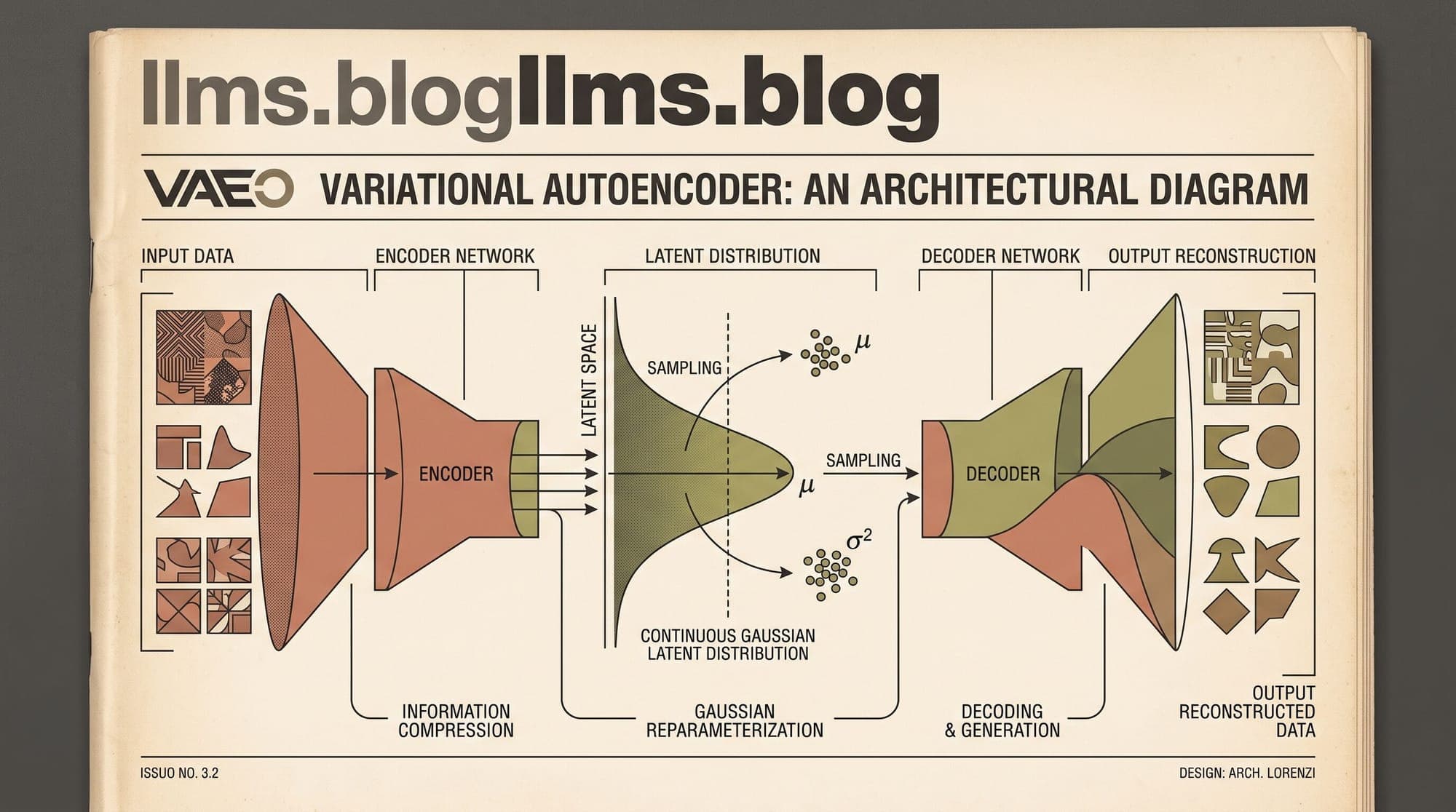
Variational Autoencoders: Mathematical Derivation of the ELBO, the Reparameterization Trick, and Mitigating Posterior Collapse

Traditional autoencoders map high-dimensional data into deterministic latent vectors. While effective for dimensionality reduction and non-linear feature compression, deterministic autoencoders fail as generative models because their latent representations lack continuous probabilistic structure. Unregularized latent spaces contain wide regions of empty space and severe discontinuities, causing decoders to produce nonsensical artifacts when sampled outside specific training points.

The Variational Autoencoder (VAE), introduced by Diederik Kingma and Max Welling (and independently by Rezende et al., 2014), transformed continuous representation learning by reformulating autoencoding within a principled probabilistic framework. Instead of mapping inputs to static points, VAEs map inputs to continuous probability distributions, optimizing a tractable surrogate objective known as the Evidence Lower Bound (ELBO).

Today, continuous VAEs form the spatial compression foundation of modern latent generative systems, including Latent Diffusion Models (Stable Diffusion), video generation backbones, and world models. Understanding the mathematical mechanics of the ELBO, the reparameterization trick, and failure modes such as posterior collapse remains essential for generative modeling.

1. The Generative Modeling Premise and Intractable Posteriors

Consider a dataset of observable samples $X = \{x^{(1)}, x^{(2)}, \dots, x^{(N)}\}$ generated by an underlying continuous random process involving unobserved continuous latent variables $z \in \mathbb{R}^d$.

The probabilistic generative model assumes a two-step generative process:

1. A latent vector $z$ is drawn from a prior distribution $p(z)$, standardly chosen as a standard isotropic Gaussian $p(z) = \mathcal{N}(z; 0, I)$.
2. An observed data vector $x \in \mathbb{R}^D$ is generated from a conditional distribution $p_\theta(x|z)$, parameterized by a neural network decoder with weights $\theta$.

The marginal likelihood of the observable data point $x$, also termed the evidence, is obtained by integrating over all possible latent states:

$$p_\theta(x) = \int p_\theta(x, z) \, dz = \int p_\theta(x|z) p(z) \, dz$$

To train this model via maximum likelihood estimation, we seek parameters $\theta$ that maximize the marginal log-likelihood:

$$\max_\theta \sum_{i=1}^N \log p_\theta(x^{(i)})$$

However, evaluating this integral directly is computationally intractable for high-dimensional latent spaces and complex non-linear decoders. Furthermore, computing the true posterior distribution over latents via Bayes' rule:

$$p_\theta(z|x) = \frac{p_\theta(x|z) p(z)}{p_\theta(x)} = \frac{p_\theta(x|z) p(z)}{\int p_\theta(x|z') p(z') \, dz'}$$

is equally intractable because the denominator requires calculating $p_\theta(x)$.

To overcome this intractability, Variational Inference introduces a parameterized recognition model (the encoder) $q_\phi(z|x)$ with parameters $\phi$, designed to approximate the true intractable posterior $p_\theta(z|x)$.

2. Mathematical Derivation of the Evidence Lower Bound (ELBO)

The variational objective can be derived directly from the Kullback-Leibler (KL) divergence between the approximate posterior $q_\phi(z|x)$ and the true posterior $p_\theta(z|x)$.

Step 1: Definition of Posterior KL Divergence

The KL divergence is defined as:

$$D_{KL}(q_\phi(z|x) \parallel p_\theta(z|x)) = \int q_\phi(z|x) \log \left( \frac{q_\phi(z|x)}{p_\theta(z|x)} \right) dz = \mathbb{E}_{q_\phi(z|x)} \left[ \log q_\phi(z|x) - \log p_\theta(z|x) \right]$$

Applying Bayes' rule to rewrite $p_\theta(z|x) = \frac{p_\theta(x, z)}{p_\theta(x)}$:

$$D_{KL}(q_\phi(z|x) \parallel p_\theta(z|x)) = \mathbb{E}_{q_\phi(z|x)} \left[ \log q_\phi(z|x) - \log p_\theta(x, z) + \log p_\theta(x) \right]$$

Step 2: Isolating the Marginal Likelihood

Because $\log p_\theta(x)$ does not depend on $z$, it can be pulled outside the expectation:

$$D_{KL}(q_\phi(z|x) \parallel p_\theta(z|x)) = \mathbb{E}_{q_\phi(z|x)} \left[ \log q_\phi(z|x) - \log p_\theta(x, z) \right] + \log p_\theta(x)$$

Rearranging terms yields:

$$\log p_\theta(x) = \mathbb{E}_{q_\phi(z|x)} \left[ \log p_\theta(x, z) - \log q_\phi(z|x) \right] + D_{KL}(q_\phi(z|x) \parallel p_\theta(z|x))$$

Step 3: Decomposing the Joint Probability

Expanding the joint density $\log p_\theta(x, z) = \log p_\theta(x|z) + \log p(z)$:

$$\log p_\theta(x) = \mathbb{E}_{q_\phi(z|x)} \left[ \log p_\theta(x|z) + \log p(z) - \log q_\phi(z|x) \right] + D_{KL}(q_\phi(z|x) \parallel p_\theta(z|x))$$

$$\log p_\theta(x) = \mathbb{E}_{q_\phi(z|x)} [\log p_\theta(x|z)] - \mathbb{E}_{q_\phi(z|x)} \left[ \log \frac{q_\phi(z|x)}{p(z)} \right] + D_{KL}(q_\phi(z|x) \parallel p_\theta(z|x))$$

$$\log p_\theta(x) = \mathbb{E}_{q_\phi(z|x)} [\log p_\theta(x|z)] - D_{KL}(q_\phi(z|x) \parallel p(z)) + D_{KL}(q_\phi(z|x) \parallel p_\theta(z|x))$$

Step 4: Establishing the Bound

Because the KL divergence is strictly non-negative ($D_{KL}(q \parallel p) \ge 0$ with equality if and only if $q = p$), dropping the final term gives a rigorous lower bound:

$$\log p_\theta(x) \ge \mathcal{L}_{\text{ELBO}}(\theta, \phi; x) = \mathbb{E}_{q_\phi(z|x)} [\log p_\theta(x|z)] - D_{KL}(q_\phi(z|x) \parallel p(z))$$

The ELBO consists of two competing terms:

• Expected Reconstruction Likelihood ($\mathbb{E}_{q_\phi(z|x)} [\log p_\theta(x|z)]$): Measures how accurately the decoder reconstructs the original input $x$ when conditioned on latents sampled from the approximate posterior.
• Prior Regularizer ($-D_{KL}(q_\phi(z|x) \parallel p(z))$): Penalizes deviations of the approximate posterior $q_\phi(z|x)$ from the Gaussian prior $p(z)$, enforcing smoothness, continuity, and preventing arbitrary clustering.

3. Closed-Form KL Divergence for Gaussian Posteriors

Under the standard VAE formulation:

• Prior: $p(z) = \mathcal{N}(z; 0, I)$
• Approximate posterior: $q_\phi(z|x) = \mathcal{N}(z; \mu(x), \text{diag}(\sigma^2(x)))$, where $\mu(x)$ and $\log \sigma^2(x)$ are deterministic outputs of the encoder network.

For two $J$-dimensional multivariate Gaussians $q(z) = \mathcal{N}(\mu, \Sigma)$ with diagonal covariance $\Sigma = \text{diag}(\sigma_1^2, \dots, \sigma_J^2)$ and standard prior $p(z) = \mathcal{N}(0, I)$, the KL divergence has a closed-form analytical expression.

The KL divergence is:

$$D_{KL}(q(z) \parallel p(z)) = \frac{1}{2} \left[ \text{tr}(\Sigma) + \mu^T \mu - J - \log \det(\Sigma) \right]$$

Expanding the trace and determinant for diagonal matrices:

$$\text{tr}(\Sigma) = \sum_{j=1}^J \sigma_j^2, \quad \mu^T \mu = \sum_{j=1}^J \mu_j^2, \quad \log \det(\Sigma) = \sum_{j=1}^J \log(\sigma_j^2)$$

Substituting these terms yields:

$$D_{KL}(q_\phi(z|x) \parallel p(z)) = -\frac{1}{2} \sum_{j=1}^J \left( 1 + \log(\sigma_j^2) - \mu_j^2 - \sigma_j^2 \right)$$

This closed-form formulation permits exact, low-variance gradient computation with respect to both $\mu(x)$ and $\log \sigma^2(x)$ without numerical integration.

4. The Reparameterization Trick: Enabling Stochastic Backpropagation

While computing the gradient of the ELBO with respect to decoder parameters $\theta$ is straightforward ($\nabla_\theta \mathcal{L}_{\text{ELBO}} = \mathbb{E}_{q_\phi(z|x)}[\nabla_\theta \log p_\theta(x|z)]$), optimizing the encoder parameters $\phi$ presents a fundamental barrier.

The gradient with respect to $\phi$ involves the distribution itself:

$$\nabla_\phi \mathbb{E}_{q_\phi(z|x)} [f(z)] = \nabla_\phi \int q_\phi(z|x) f(z) \, dz$$

Score Function Estimator (REINFORCE)

The general black-box variational inference method uses the log-derivative trick:

$$\nabla_\phi \mathbb{E}_{q_\phi(z|x)} [f(z)] = \mathbb{E}_{q_\phi(z|x)} \left[ f(z) \nabla_\phi \log q_\phi(z|x) \right]$$

While unbiased, this score function estimator exhibits catastrophic variance across mini-batches, rendering gradient descent in deep architectures unstable without complex variance reduction baselines.

The Pathwise Gradient / Reparameterization Transformation

Kingma and Welling resolved this by reparameterizing the random variable $z \sim q_\phi(z|x)$ as a deterministic function of the input $x$, encoder parameters $\phi$, and an auxiliary independent noise variable $\epsilon$:

$$z = g_\phi(x, \epsilon) = \mu(x) + \sigma(x) \odot \epsilon, \quad \text{where } \epsilon \sim \mathcal{N}(0, I)$$

Here, $\odot$ denotes element-wise multiplication.

Under this transformation, the expectation with respect to $q_\phi(z|x)$ transforms into an expectation over the parameter-free distribution $p(\epsilon)$:

$$\mathbb{E}_{q_\phi(z|x)} [f(z)] = \mathbb{E}_{p(\epsilon)} \left[ f(g_\phi(x, \epsilon)) \right]$$

Now the gradient operator $\nabla_\phi$ moves inside the integral directly:

$$\nabla_\phi \mathbb{E}_{q_\phi(z|x)} [f(z)] = \mathbb{E}_{p(\epsilon)} \left[ \nabla_z f(z) \cdot \nabla_\phi g_\phi(x, \epsilon) \right] = \mathbb{E}_{p(\epsilon)} \left[ \nabla_z f(z) \cdot \left( \nabla_\phi \mu(x) + \epsilon \odot \nabla_\phi \sigma(x) \right) \right]$$

A single Monte Carlo sample $\epsilon \sim \mathcal{N}(0, I)$ per data point in a mini-batch provides an unbiased, low-variance gradient estimate suitable for standard stochastic backpropagation.

5. The Pathology of Posterior Collapse

A central challenge in training continuous VAEs is posterior collapse (also termed latent variable collapse).

Mathematical Definition

Posterior collapse occurs when the approximate posterior becomes independent of the input and collapses to the prior:

$$q_\phi(z|x) \approx p(z) = \mathcal{N}(0, I) \quad \forall x$$

When this occurs:

• The KL divergence drops to zero: $D_{KL}(q_\phi(z|x) \parallel p(z)) \to 0$.
• The mutual information between inputs and latents approaches zero: $I(X; Z) = \mathbb{E}_{p(x)}[D_{KL}(q_\phi(z|x) \parallel q(z))] \to 0$.
• The decoder completely ignores the latent code $z$, modeling $p_\theta(x|z) \approx p(x)$ purely through internal autoregressive or local representations.

Why Posterior Collapse Happens

Posterior collapse is particularly acute when the decoder possesses high expressive capacity (e.g., PixelCNN, autoregressive RNNs, or masked Transformers) as studied by Bowman et al. (2015) and Chen et al. (2016).

Early in training:

1. The encoder output $\mu(x)$ and $\sigma(x)$ are noisy and uninformative.
2. The expressive decoder learns to predict $x$ using its own contextual conditioning (e.g., previous tokens in text or neighboring pixels in images).
3. The optimizer quickly realizes it can minimize the total loss by setting $D_{KL} = 0$ (setting $\mu \to 0, \sigma \to 1$) without sacrificing reconstruction performance.
4. Once $z$ carries no signal, gradients $\nabla_z \log p_\theta(x|z)$ vanish, permanently locking the encoder into an uninformative prior match.

Diagnostic Metrics

To detect posterior collapse during training, practitioners track Active Units (AU) (Burda et al., 2015):

$$\text{AU} = \left\{ j \in \{1, \dots, J\} \;\middle|\; \text{Var}_{x \sim \mathcal{D}} \left( \mathbb{E}_{q_\phi(z_j|x)}[z_j] \right) > \delta \right\}$$

where $\delta$ is a variance threshold (typically $0.01$). If the count of active units drops toward zero, the latent dimensions have collapsed.

6. Modern Mitigation Strategies

Multiple techniques have been developed to preserve latent capacity and prevent collapse:

1. $\beta$-VAE and Controlled Capacity

Higgins et al. (2017) introduced $\beta$-VAE, adding a scaling factor $\beta$ to the KL regularization term:

$$\mathcal{L}_{\beta\text{-VAE}} = \mathbb{E}_{q_\phi(z|x)} [\log p_\theta(x|z)] - \beta \, D_{KL}(q_\phi(z|x) \parallel p(z))$$

• Setting $\beta < 1$ weakens prior pressure, preventing collapse and prioritizing reconstruction fidelity.
• Setting $\beta > 1$ enforces statistical independence across latent dimensions, encouraging disentangled representations.

Burgess et al. (2018) refined this with progressive capacity annealing:

$$\mathcal{L} = \mathbb{E}_{q_\phi(z|x)} [\log p_\theta(x|z)] - \gamma \left| D_{KL}(q_\phi(z|x) \parallel p(z)) - C \right|$$

where channel capacity $C$ is gradually increased from $0$ to target bits during training.

2. KL Annealing and Cyclical Schedules

Bowman et al. (2015) proposed linear KL annealing, starting $\beta = 0$ and linearly ramping to $\beta = 1$ over warmup steps. This gives the encoder time to learn meaningful semantic features before the prior constraint takes effect.

Fu et al. (2019) improved upon linear annealing with Cyclical Annealing, repeating the $\beta = 0 \to 1$ schedule across multiple cycles throughout training to periodically free latent space and reactivate collapsed dimensions.

3. Free Bits / Minimum Description Length Thresholding

Kingma et al. (2016) introduced the Free Bits heuristic, which enforces a minimum KL penalty $\tau$ per latent dimension:

$$\mathcal{L}_{\text{free-bits}} = \mathbb{E}_{q_\phi(z|x)} [\log p_\theta(x|z)] - \sum_{j=1}^J \max \left( \tau, D_{KL}(q_\phi(z_j|x) \parallel p(z_j)) \right)$$

This prevents dimensions with small KL contributions from being pushed all the way to zero, ensuring each dimension maintains a minimum information threshold.

7. Comparative Architectural Paradigms

Different latent generative architectures address representation capacity, likelihood evaluation, and training dynamics through distinct trade-offs:

• Standard VAE (Kingma & Welling, 2013): Employs a continuous Gaussian latent space $\mathbb{R}^d$ optimized with standard ELBO ($\beta = 1$). Provides approximate likelihood via lower bounding, but susceptible to posterior collapse with powerful autoregressive decoders.
• $\beta$-VAE (Higgins et al., 2017): Introduces adjustable $\beta$ weighting on the KL divergence. $\beta > 1$ forces axis-aligned factor disentanglement at the expense of reconstruction sharpness, while $\beta < 1$ prioritizes reconstruction fidelity.
• VQ-VAE / VQ-VAE-2 (van den Oord et al., 2017): Replaces continuous Gaussians with a discrete learnable codebook. Completely circumvents posterior collapse and variance sampling issues, but requires straight-through gradient estimation and two-stage autoregressive prior learning.
• Hierarchical VAE (NVAE / VDVAE): Utilizes deep ladders of continuous Gaussian latents with residual cellular structures and bidirectional skip connections, yielding high-resolution density estimation.
• Continuous Normalizing Flows (Lipman et al., 2022): Maps distributions via invertible ODE vector fields without dimensionality reduction, enabling exact likelihood computation at the cost of integration compute.
• Latent Diffusion AutoencoderKL (Rombach et al., 2022): Continuous spatial latent map $\mathbb{R}^{h/8 \times w/8 \times c}$ trained with perceptual patch LPIPS loss and very small KL weighting ($\beta \approx 10^{-6}$), serving as the continuous perceptual compression layer for Stable Diffusion and Flux.

8. Reference Implementation: PyTorch VAE with Free Bits and KL Annealing

Below is a complete, self-contained PyTorch implementation demonstrating the encoder, Gaussian reparameterization, closed-form KL divergence, and the Free Bits regularization objective.

import torch
import torch.nn as nn
import torch.nn.functional as F

class VariationalAutoencoder(nn.Module):
    def __init__(self, input_dim: int, hidden_dim: int, latent_dim: int):
        super().__init__()
        self.latent_dim = latent_dim
        
        # Encoder Network
        self.encoder_backbone = nn.Sequential(
            nn.Linear(input_dim, hidden_dim),
            nn.SiLU(),
            nn.Linear(hidden_dim, hidden_dim),
            nn.SiLU()
        )
        self.fc_mu = nn.Linear(hidden_dim, latent_dim)
        self.fc_logvar = nn.Linear(hidden_dim, latent_dim)
        
        # Decoder Network
        self.decoder = nn.Sequential(
            nn.Linear(latent_dim, hidden_dim),
            nn.SiLU(),
            nn.Linear(hidden_dim, hidden_dim),
            nn.SiLU(),
            nn.Linear(hidden_dim, input_dim)
        )

    def encode(self, x: torch.Tensor):
        h = self.encoder_backbone(x)
        mu = self.fc_mu(h)
        logvar = self.fc_logvar(h)
        return mu, logvar

    def reparameterize(self, mu: torch.Tensor, logvar: torch.Tensor) -> torch.Tensor:
        """
        Applies the pathwise gradient reparameterization trick.
        z = mu + sigma * epsilon, where epsilon ~ N(0, I)
        """
        if self.training:
            std = torch.exp(0.5 * logvar)
            eps = torch.randn_like(std)
            return mu + eps * std
        return mu

    def decode(self, z: torch.Tensor) -> torch.Tensor:
        return self.decoder(z)

    def forward(self, x: torch.Tensor):
        mu, logvar = self.encode(x)
        z = self.reparameterize(mu, logvar)
        recon_x = self.decode(z)
        return recon_x, mu, logvar


def compute_vae_loss(
    recon_x: torch.Tensor,
    x: torch.Tensor,
    mu: torch.Tensor,
    logvar: torch.Tensor,
    beta: float = 1.0,
    free_bits_nats: float = 0.0
) -> dict[str, torch.Tensor]:
    """
    Computes Gaussian ELBO loss with optional beta-scaling and free bits per dimension.
    """
    # 1. Reconstruction Loss (Mean Squared Error)
    recon_loss = F.mse_loss(recon_x, x, reduction="none").sum(dim=-1)

    # 2. Analytical Closed-Form KL Divergence per dimension:
    # D_KL = -0.5 * sum(1 + log(sigma^2) - mu^2 - sigma^2)
    kl_per_dim = -0.5 * (1.0 + logvar - mu.pow(2) - logvar.exp())

    if free_bits_nats > 0.0:
        # Free Bits / Minimum Description Length constraint
        kl_per_dim = torch.clamp(kl_per_dim, min=free_bits_nats)

    kl_loss = kl_per_dim.sum(dim=-1)

    total_loss = (recon_loss + beta * kl_loss).mean()

    return {
        "loss": total_loss,
        "recon_loss": recon_loss.mean(),
        "kl_loss": kl_loss.mean()
    }

9. Latent Spaces in Frontier Diffusion Models

The fundamental principles of continuous VAEs remain at the core of current frontier generative AI. In Latent Diffusion Models and subsequent architectures like Stable Diffusion 3 and Flux:

1. An initial AutoencoderKL stage trains a deep continuous VAE with spatial downsampling factors (typically $f=8$).
2. A high-resolution $1024 \times 1024 \times 3$ image is compressed into a continuous latent tensor $z \in \mathbb{R}^{128 \times 128 \times 16}$.
3. A light KL penalty ($\beta \approx 10^{-6}$) prevents latent variance explosion while preserving high-frequency perceptual details via LPIPS patch losses.
4. The downstream Diffusion Transformer or U-Net operates entirely within this smooth, low-dimensional Gaussian manifold.

By turning continuous inference into a tractable optimization problem via the ELBO and the reparameterization trick, the VAE framework established the foundational bridge between probabilistic Bayesian inference and modern deep generative architectures.

Sources

• Auto-Encoding Variational Bayes (Kingma & Welling, ICLR 2014)
• Stochastic Backpropagation and Approximate Inference in Deep Generative Models (Rezende et al., ICML 2014)
• $\beta$-VAE: Learning Basic Visual Concepts with a Constrained Variational Framework (Higgins et al., ICLR 2017)
• Generating Sentences from a Continuous Space (Bowman et al., CoNLL 2016)
• Variational Lossy Autoencoder (Chen et al., ICLR 2017)
• Understanding Disentangling in $\beta$-VAE (Burgess et al., NeurIPS 2018)
• Cyclical Annealing Schedule: A Simple Approach to Mitigating Posterior Collapse (Fu et al., NAACL 2019)
• High-Resolution Image Synthesis with Latent Diffusion Models (Rombach et al., CVPR 2022)