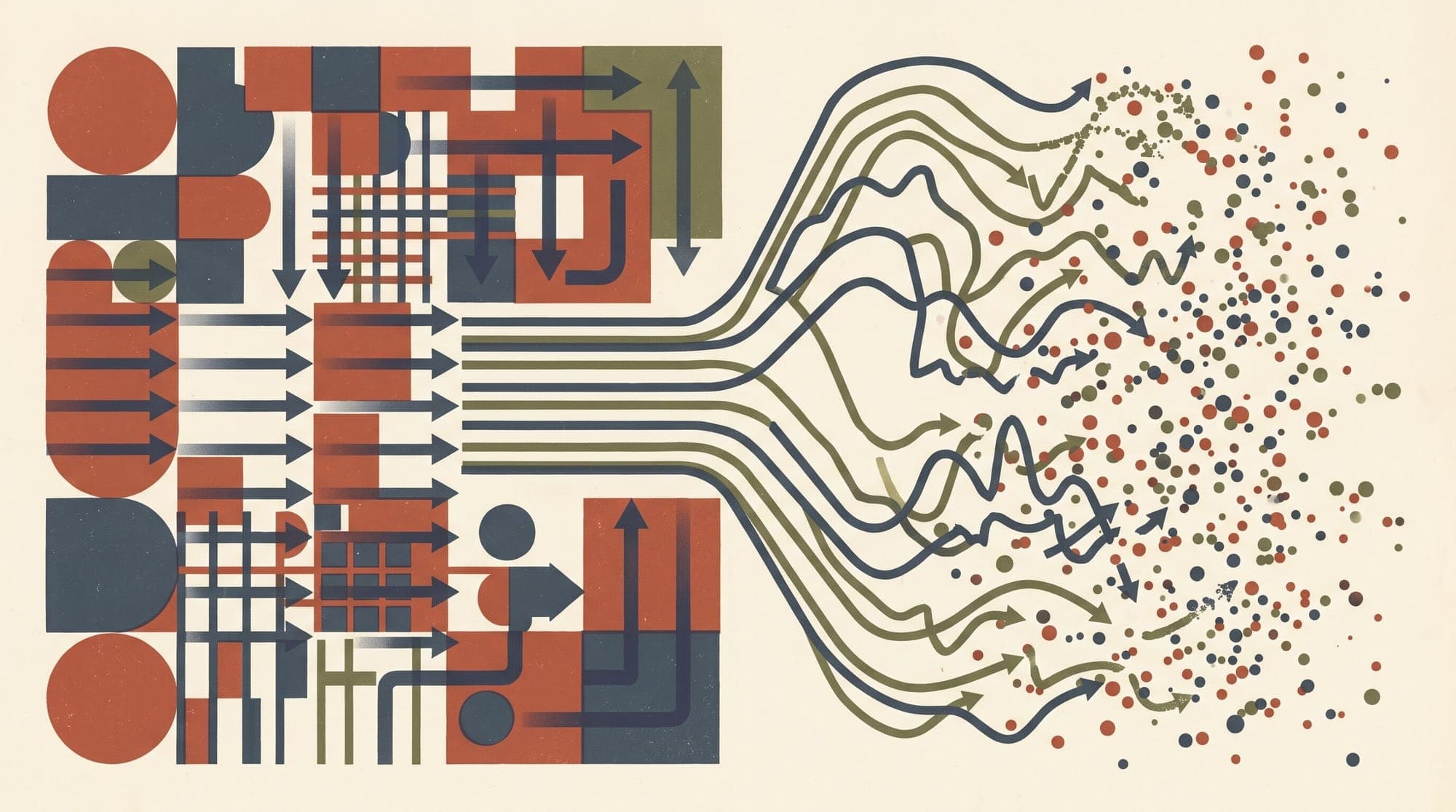
Score-Based Generative Modeling via Stochastic Differential Equations: How Continuous SDEs and Score Matching Unify Diffusion Models

Diffusion and score-based models represent one of the foundational paradigms of modern generative artificial intelligence, underpinning systems across image synthesis, video generation, audio modeling, and continuous multimodal representations. For years, generative diffusion was approached from two distinct perspectives: discrete-step denoising diffusion probabilistic models (DDPM) pioneered by Sohl-Dickstein et al. and Ho et al., and score matching with Langevin dynamics (SMLD / NCSN) introduced by Song and Ermon.

In 2020, Song et al. unified both frameworks under the continuous-time mathematical theory of Stochastic Differential Equations (SDEs). By treating the noise corruption and generative reconstruction processes as continuous paths governed by forward and reverse-time Itô SDEs, the framework revealed that discrete diffusion models are numerical discretizations of underlying continuous processes.

This continuous formulation unlocked several practical capabilities: exact likelihood computation via continuous normalizing flows, deterministic sampling via the Probability Flow ODE, predictor-corrector sampling architectures, and flexible controllable generation.

1. The Core Formulation: Forward and Reverse-Time SDEs

Traditional diffusion models define a discrete Markov chain over $T$ distinct time steps $\{x_0, x_1, \dots, x_T\}$ . In the continuous limit as $T \to \infty$ and the step size $\Delta t \to 0$ , the forward corruption process evolves according to an Itô Stochastic Differential Equation:

$dx = f(x, t) dt + g(t) dw$

In this equation:

$x(t) \in \mathbb{R}^d$ represents the continuous state vector indexed by continuous time $t \in [0, T]$ .
$f(x, t): \mathbb{R}^d \times [0, T] \to \mathbb{R}^d$ is the drift coefficient, governing deterministic state shifts over time.
$g(t): [0, T] \to \mathbb{R}$ is the diffusion coefficient, modulating the scale of injected stochastic noise.
$w \in \mathbb{R}^d$ denotes standard Brownian motion (a Wiener process), with infinitesimal increment $dw \sim \mathcal{N}(0, I dt)$ .

As $t$ evolves from $0$ to $T$ , the data distribution $p_0(x)$ is smoothly transformed into a tractable prior distribution $p_T(x)$ , typically an isotropic standard Gaussian distribution $\mathcal{N}(0, \sigma_{\max}^2 I)$ or $\mathcal{N}(0, I)$ .

Continuous-time forward SDE diffusion, reverse-time score-guided generation, and deterministic Probability Flow ODE trajectories

The Reverse-Time SDE

To generate new samples, one must reverse the continuous diffusion process from $t = T$ back to $t = 0$ . Using classical results in stochastic calculus established by Brian D. O. Anderson (1982)90051-5), the reverse of an Itô diffusion process is itself an Itô diffusion running backward in time:

$dx = \left[ f(x, t) - g(t)^2 \nabla_x \log p_t(x) \right] dt + g(t) d\bar{w}$

Here, $dt$ represents an infinitesimal negative time increment (marching backward from $T$ to $0$ ), $d\bar{w}$ denotes a reverse-time standard Brownian motion, and $\nabla_x \log p_t(x)$ is the score function: the spatial gradient of the log-probability density of the marginal distribution $p_t(x)$ at time $t$ .

The critical insight of score-based modeling is that the drift $f(x, t)$ and diffusion $g(t)$ are predetermined analytical design choices. The only unknown quantity required to simulate the reverse process is the time-dependent score function $\nabla_x \log p_t(x)$ .

2. Unifying DDPM and SMLD in Continuous Time

The continuous SDE framework demonstrates that discrete diffusion algorithms are simply specific parameterizations of drift and diffusion coefficients:

Variance Exploding (VE) SDE (Continuous SMLD)

Score Matching with Langevin Dynamics (SMLD / NCSN) perturbs data with a sequence of growing Gaussian noise variances $\sigma_1 < \sigma_2 < \dots < \sigma_N$ . In continuous time, this corresponds to a process where the drift is zero and the variance grows monotonically:

$f(x, t) = 0, \quad g(t) = \sqrt{\frac{d[\sigma^2(t)]}{dt}}$

The resulting VE-SDE is:

$dx = \sqrt{\frac{d[\sigma^2(t)]}{dt}} dw$

The perturbation kernel from $0$ to $t$ is Gaussian:

$p_{0t}(x(t) \mid x(0)) = \mathcal{N}\left(x(t); x(0), \left(\sigma^2(t) - \sigma^2(0)\right) I\right)$

Because the state variance diverges as $t \to T$ , this formulation is termed Variance Exploding.

Variance Preserving (VP) SDE (Continuous DDPM)

Denoising Diffusion Probabilistic Models (DDPM) scale down the input vector at each step while adding scaled noise to keep the total variance bounded:

$x_i = \sqrt{1 - \beta_i} x_{i-1} + \sqrt{\beta_i} z_{i-1}$

Taking the continuous limit where $\beta_i = \beta(t) \Delta t$ , the drift and diffusion become:

$f(x, t) = -\frac{1}{2} \beta(t) x, \quad g(t) = \sqrt{\beta(t)}$

The resulting VP-SDE is:

$dx = -\frac{1}{2} \beta(t) x dt + \sqrt{\beta(t)} dw$

The transition kernel satisfies:

$p_{0t}(x(t) \mid x(0)) = \mathcal{N}\left(x(t); x(0) e^{-\frac{1}{2}\int_0^t \beta(s)ds}, \left(1 - e^{-\int_0^t \beta(s)ds}\right) I\right)$

If the initial data variance is normalized to 1, the total variance remains exactly 1 across all $t$ , hence Variance Preserving.

Sub-VP SDE

Song et al. introduced the sub-VP SDE, which modifies the diffusion coefficient:

$g(t) = \sqrt{\beta(t) \left(1 - e^{-2\int_0^t \beta(s)ds}\right)}$

This ensures that the variance at any intermediate time $t$ is strictly upper-bounded by the VP-SDE variance, yielding empirically superior negative log-likelihood (NLL) bounds.

3. Training the Score Network via Denoising Score Matching

Direct computation of $\nabla_x \log p_t(x)$ is impossible because the true marginal data density $p_t(x) = \int p_0(x_0) p_{0t}(x \mid x_0) dx_0$ is intractable.

However, by extending Vincent's (2011) denoising score matching to continuous time, we train a neural network $s_\theta(x, t)$ to approximate the score of the tractable transition kernel $p_{0t}(x(t) \mid x(0))$ .

The continuous denoising score matching loss objective is:

$\mathcal{L}(\theta) = \mathbb{E}_{t \sim \mathcal{U}(\epsilon, T)} \mathbb{E}_{x(0) \sim p_0} \mathbb{E}_{x(t) \sim p_{0t}(x(t) \mid x(0))} \left[ \lambda(t) \left\| s_\theta(x(t), t) - \nabla_{x(t)} \log p_{0t}(x(t) \mid x(0)) \right\|_2^2 \right]$

where $\lambda(t): [0, T] \to \mathbb{R}^+$ is a positive weighting function, typically chosen as $\lambda(t) \propto \frac{1}{\mathbb{E}\left[\|\nabla_{x(t)} \log p_{0t}(x(t) \mid x(0))\|_2^2\right]}$ to balance loss magnitudes across different noise scales.

Equivalence to Noise Prediction

Because $p_{0t}(x(t) \mid x(0))$ is Gaussian with mean $\mu(x(0), t)$ and variance $\sigma^2(t) I$ , its ground-truth score has a simple analytical form:

$\nabla_{x(t)} \log p_{0t}(x(t) \mid x(0)) = -\frac{x(t) - \mu(x(0), t)}{\sigma^2(t)} = -\frac{\epsilon}{\sigma(t)}$

where $\epsilon \sim \mathcal{N}(0, I)$ is the standard Gaussian noise vector used to generate $x(t)$ .

Thus, predicting the score function $s_\theta(x(t), t)$ is mathematically equivalent to predicting the injected noise $\epsilon_\theta(x(t), t) = -\sigma(t) s_\theta(x(t), t)$ , establishing an exact identity between score matching and DDPM objective formulations.

4. The Probability Flow ODE and Exact Likelihoods

Every Itô SDE of the form $dx = f(x, t)dt + g(t)dw$ possesses an associated deterministic Ordinary Differential Equation (ODE), termed the Probability Flow ODE:

$\frac{dx}{dt} = f(x, t) - \frac{1}{2} g(t)^2 \nabla_x \log p_t(x)$

The Probability Flow ODE shares the exact same marginal probability densities $p_t(x)$ as the stochastic SDE for all $t \in [0, T]$ .

+-------------------------------------------------------------+
|                     Forward SDE                             |
|           dx = f(x, t)dt + g(t)dw (adds noise)              |
+------------------------------+------------------------------+
                               |
                               v
+-------------------------------------------------------------+
|                  Learned Score Function                     |
|                 s_theta(x, t) ~= grad_x log p_t(x)          |
+------------------------------+------------------------------+
                               |
               +---------------+---------------+
               |                               |
               v                               v
+-----------------------------+ +-----------------------------+
|      Reverse-Time SDE       | |    Probability Flow ODE     |
| dx = [f - g^2 s_theta]dt    | | dx/dt = f - 0.5 g^2 s_theta |
|         + g d_w_bar         | |                             |
|  (Stochastic generation)    | |  (Deterministic trajectory) |
+-----------------------------+ +-----------------------------+
                                               |
                               +---------------+---------------+
                               |                               |
                               v                               v
                +-----------------------------+ +-------------+
                | Continuous Normalizing Flow | |  Fast ODE   |
                |   Exact Log-Likelihood      | |   Solvers   |
                | Hutchinson Trace Estimator  | | (Dopri5/RK4)|
                +-----------------------------+ +-------------+

Exact Log-Likelihood via Continuous Normalizing Flows

Because the Probability Flow ODE defines a deterministic, invertible mapping between data space $x(0)$ and latent space $x(T)$ , it can be treated as a Continuous Normalizing Flow (CNF).

Using the instantaneous change of variables formula, the exact log-likelihood of any data point $x(0)$ can be computed by integrating the divergence of the drift field over time:

$\log p_0(x(0)) = \log p_T(x(T)) + \int_0^T \nabla \cdot \tilde{f}_\theta(x(t), t) dt$

where $\tilde{f}_\theta(x, t) = f(x, t) - \frac{1}{2} g(t)^2 s_\theta(x, t)$ .

The divergence $\nabla \cdot \tilde{f}_\theta$ involves computing the trace of the Jacobian matrix $\text{Tr}\left(\frac{\partial \tilde{f}_\theta}{\partial x}\right)$ , which is computed efficiently using the Skilling-Hutchinson trace estimator:

$\nabla \cdot \tilde{f}_\theta(x, t) = \mathbb{E}_{v \sim \mathcal{N}(0, I)} \left[ v^T \left( \nabla_x \tilde{f}_\theta(x, t) \right) v \right]$

This requires only a single vector-Jacobian product (VJP) per step via automatic differentiation, turning score models into exact density estimators without partition function intractability.

5. Sampling Architectures: Predictor-Corrector Framework

The continuous framework allows decoupling model training from the choice of numerical solvers. During inference, one can use standard high-order numerical ODE solvers (such as Dormand-Prince / Dopri5 or Runge-Kutta 4) or hybrid Predictor-Corrector (PC) samplers.

A Predictor-Corrector sampler alternates between two complementary operations at each discrete time step $t_i$ :

Predictor Step: Uses a numerical SDE solver (such as Euler-Maruyama or Reverse Diffusion) to advance the state from $t_i$ to $t_{i-1}$ , predicting the coarse evolution of the sample.
Corrector Step: Runs several steps of score-based Markov Chain Monte Carlo (MCMC), such as annealed Langevin dynamics, at fixed time $t_{i-1}$ :

$x \leftarrow x + \frac{\epsilon_k}{2} s_\theta(x, t_{i-1}) + \sqrt{\epsilon_k} z, \quad z \sim \mathcal{N}(0, I)$

The corrector step acts as an error-correction mechanism, pulling the trajectory back toward the high-density regions of the intermediate marginal distribution $p_{t_{i-1}}(x)$ whenever numerical discretization error accumulates.

import torch

def euler_maruyama_predictor_step(x, t, dt, f_fn, g_fn, score_fn):
    """Executes a single reverse-time Euler-Maruyama SDE step."""
    drift = f_fn(x, t) - (g_fn(t) ** 2) * score_fn(x, t)
    diffusion = g_fn(t)
    z = torch.randn_like(x) if t > 0 else torch.zeros_like(x)
    # Note: dt is negative when stepping backwards from T to 0
    x_prev = x + drift * dt + diffusion * torch.sqrt(torch.abs(dt)) * z
    return x_prev

def langevin_corrector_step(x, t, score_fn, r=0.16, snr=0.16):
    """Executes a single Langevin dynamics corrector step at fixed time t."""
    grad = score_fn(x, t)
    noise = torch.randn_like(x)
    
    # Calculate step size based on Signal-to-Noise Ratio (SNR)
    grad_norm = torch.norm(grad.reshape(grad.shape[0], -1), dim=-1).mean()
    noise_norm = torch.norm(noise.reshape(noise.shape[0], -1), dim=-1).mean()
    step_size = 2 * (snr * noise_norm / grad_norm) ** 2
    
    x = x + step_size * grad + torch.sqrt(2 * step_size) * noise
    return x

6. Structural Trade-Offs and Architectural Impact

The transition to continuous score SDEs reshaped generative modeling research across several axes:

| Feature | Discrete Diffusion (DDPM / SMLD) | Continuous Score SDEs | | :--- | :--- | :--- | | Time Representation | Discrete index $t \in \{1, \dots, N\}$ | Continuous variable $t \in [0, T]$ | | Sampling Mechanism | Fixed step-by-step Markov reverse chain | Flexible SDE, ODE, or Predictor-Corrector solvers | | Sample Trajectory | Purely stochastic | Choice between stochastic (SDE) and deterministic (ODE) | | Likelihood Evaluation | Variational Lower Bound (ELBO) | Exact log-likelihood via Probability Flow ODE | | Latent Inversion | Approximate or heuristic (DDIM) | Exact bidirectional encoding via ODE flow | | Step-Count Flexibility | Requires fixed retraining or resampling schedule | Arbitrary number of function evaluations (NFEs) at inference |

Descendants and Modern Offshoots

The mathematical rigor established by continuous score SDEs provided the direct theoretical foundation for several subsequent breakthroughs:

Flow Matching and Continuous Normalizing Flows: Lipman et al. (2022) generalized score SDEs by formulating generative modeling as regressing arbitrary continuous velocity vector fields along optimal transport paths, removing the restriction to isotropic Gaussian diffusion.
Consistency Models: Song et al. (2023) used the trajectories of the Probability Flow ODE to enforce a self-consistency mapping from any point on the ODE path directly to its origin $x(0)$ , enabling single-step and few-step generation.
Diffusion Transformers (DiT): Peebles and Xie (2022) scaled the underlying score network from standard U-Nets to vision transformers, operating on tokenized patch representations conditioned on continuous time embeddings $t$ .

By recasting diffusion from discrete heuristic noise steps into continuous stochastic calculus, score-based SDEs established a unified theoretical foundation that continues to govern modern generative architectures.