Kolmogorov-Arnold Networks: How Learnable Edge Splines Challenge the Multi-Layer Perceptron

For over three decades, the foundational building block of deep neural networks has remained essentially unchanged: the Multi-Layer Perceptron (MLP). In standard transformer feed-forward blocks, convolutional networks, and deep classifiers, MLPs alternate linear matrix multiplications ($\mathbf{W}\mathbf{x}$) with fixed, point-wise non-linear activation functions (such as ReLU, GELU, or SwiGLU). Under this paradigm, all non-linearity occurs at the nodes (neurons), while connections (weights) are purely linear scalars.

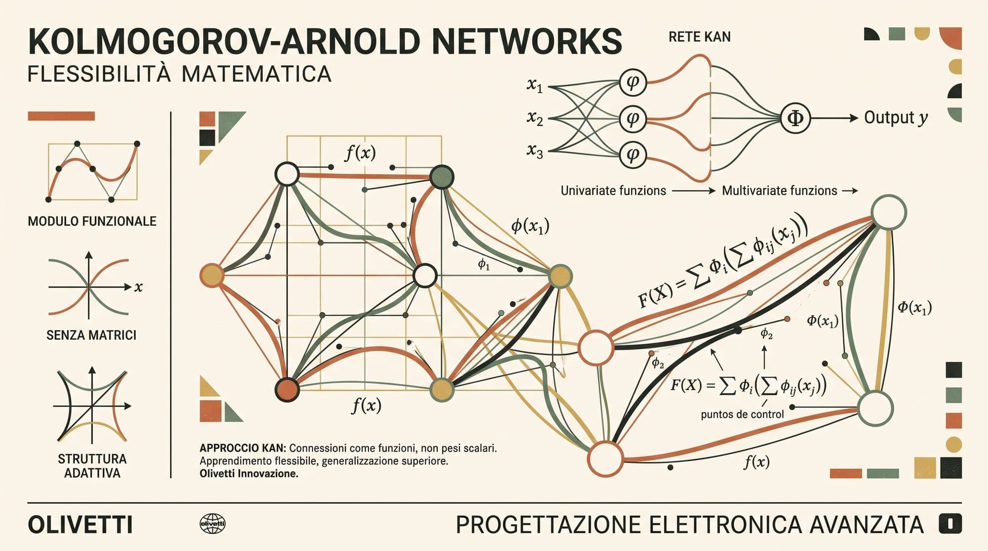
In 2024, researchers from MIT, Caltech, and Northeastern University proposed Kolmogorov-Arnold Networks (KANs), an alternative architecture that inverts this structural assumption. In a KAN, nodes do not apply activation functions; they act as simple linear accumulators that sum incoming signals. The non-linear transformations are instead moved entirely onto the network edges, where every connection is parameterized as a learnable univariate spline function.

Rooted in classical mathematical approximation theory, KANs achieve faster neural scaling exponents, provide resistance to catastrophic forgetting, and enable exact symbolic extraction for scientific discovery. However, their reliance on non-uniform spline evaluation presents fundamental execution challenges on modern hardware optimized for dense matrix multiplication.

1. Theoretical Foundations: The Kolmogorov-Arnold Representation Theorem

The mathematical basis of KANs traces back to David Hilbert's 13th problem, posed in 1900, which questioned whether any continuous function of three variables could be expressed as a composition of continuous functions of two variables. In 1957, Soviet mathematicians Andrey Kolmogorov and Vladimir Arnold proved a stronger result known as the Kolmogorov-Arnold Representation Theorem (KAT).

The theorem proves that any continuous multivariate function $f: [0, 1]^n \to \mathbb{R}$ defined on a bounded domain can be written as a finite composition of continuous functions of a single variable and the binary operation of addition:

$$f(\mathbf{x}) = f(x_1, \dots, x_n) = \sum_{q=1}^{2n+1} \Phi_q \left( \sum_{p=1}^n \phi_{q,p}(x_p) \right)$$

where $\phi_{q,p}: [0, 1] \to \mathbb{R}$ and $\Phi_q: \mathbb{R} \to \mathbb{R}$ are continuous 1D univariate functions.

The theoretical implication of KAT is profound: true multivariate functions do not fundamentally exist; every high-dimensional relationship can be reduced to single-variable transformations combined through addition.

Why Early Machine Learning Abandoned KAT

Despite its mathematical elegance, early neural network researchers in the late 1980s and 1990s—including Girosi and Poggio (1989)—abandoned the Kolmogorov-Arnold representation in favor of the Universal Approximation Theorem for MLPs (Cybenko 1989, Hornik 1991).

The primary obstacle was smoothness:

1. Pathological 1D Functions: For arbitrary continuous multivariate functions, the theoretical inner functions $\phi_{q,p}$ constructed in the original 2-layer KAT proof can be non-smooth, nowhere-differentiable, or fractal.
2. Optimization Collapse: Because early formulations restricted the architecture strictly to a rigid depth-2 graph with $(2n+1)$ hidden units, standard gradient-based optimization failed to learn these highly jagged functions.
3. The Rise of MLPs: MLPs side-stepped this difficulty by utilizing fixed, smooth (or sub-differentiable) activations and distributing complexity across large matrices of linear weights.

2. Generalizing KAT to Arbitrary Depth and Width

The core insight introduced by Liu et al. (2024) was that the limitations of classical KAT stemmed from its rigid two-layer constraint. In real-world physical systems and natural data distributions, target functions possess hierarchical, compositional smoothness. By generalizing KAT to arbitrary depths and widths, deep KANs decompose complex functions across multiple smooth intermediate layers.

Defining a KAN Layer

A KAN layer with $n_{\text{in}}$ inputs and $n_{\text{out}}$ outputs is defined as a matrix of 1D parameterized functions:

$$\mathbf{\Phi} = \{ \phi_{q,p} \}, \quad p = 1, \dots, n_{\text{in}}, \quad q = 1, \dots, n_{\text{out}}$$

For an input vector $\mathbf{x} = [x_1, x_2, \dots, x_{n_{\text{in}}}]^T$, the output vector $\mathbf{y} \in \mathbb{R}^{n_{\text{out}}}$ is computed by evaluating each activation function along its respective edge and summing at the destination node:

$$y_q = \sum_{p=1}^{n_{\text{in}}} \phi_{q,p}(x_p)$$

In matrix form:

$$\mathbf{x}_{l+1} = \mathbf{\Phi}_l(\mathbf{x}_l) = \begin{pmatrix} \phi_{l,1,1}(\cdot) & \phi_{l,1,2}(\cdot) & \cdots & \phi_{l,1,n_l}(\cdot) \\ \phi_{l,2,1}(\cdot) & \phi_{l,2,2}(\cdot) & \cdots & \phi_{l,2,n_l}(\cdot) \\ \vdots & \vdots & \ddots & \vdots \\ \phi_{l,n_{l+1},1}(\cdot) & \phi_{l,n_{l+1},2}(\cdot) & \cdots & \phi_{l,n_{l+1},n_l}(\cdot) \end{pmatrix} \mathbf{x}_l$$

A deep KAN with $L$ layers and layer widths $[n_0, n_1, \dots, n_L]$ is simply the function composition of these layer matrices:

$$\text{KAN}(\mathbf{x}) = (\mathbf{\Phi}_{L-1} \circ \mathbf{\Phi}_{L-2} \circ \dots \circ \mathbf{\Phi}_1 \circ \mathbf{\Phi}_0)\mathbf{x}$$

Whereas an MLP interleaves linear operations $\mathbf{W}_l$ and fixed activations $\sigma$:

$$\text{MLP}(\mathbf{x}) = (\mathbf{W}_{L-1} \circ \sigma \circ \mathbf{W}_{L-2} \circ \sigma \circ \dots \circ \mathbf{W}_0)\mathbf{x}$$

KANs merge the linear scaling and non-linear transformation into a unified edge operator $\mathbf{\Phi}_l$.

MLP Layer (Node-Activated):
x₁ ───[w₁₁]───( + )───[ σ(·) ]───> y₁
x₂ ───[w₁₂]───╯

KAN Layer (Edge-Activated):
x₁ ───[ ϕ₁₁(x₁) ]───( + )────────> y₁
x₂ ───[ ϕ₁₂(x₂) ]───╯

3. Mathematical Parameterization: B-Splines and Residual Bases

To make KAN layers differentiable and trainable via standard backpropagation, each edge function $\phi(x)$ is parameterized as a combination of a smooth base function and a localized B-spline curve:

$$\phi(x) = w \cdot \left( b(x) + \text{spline}(x) \right)$$

1. Residual Base Function

The base function $b(x)$ provides a continuous global gradient highway, avoiding vanishing gradients during initialization:

$$b(x) = \text{SiLU}(x) = \frac{x}{1 + e^{-x}}$$

A scalar weight $w$ scales the overall magnitude, initialized via Xavier initialization.

2. B-Spline Basis

The flexible non-linear component is represented as a linear combination of B-spline basis functions of order $k$ (typically cubic, $k=3$) defined across $G$ grid intervals ($G+1$ knot points):

$$\text{spline}(x) = \sum_{i=0}^{G+k-1} c_i B_i(x)$$

The B-spline basis functions $B_i(x)$ are computed recursively using the Cox-de Boor recursion formula:

$$B_{i,0}(x) = \begin{cases} 1 & \text{if } t_i \le x < t_{i+1} \\ 0 & \text{otherwise} \end{cases}$$

$$B_{i,k}(x) = \frac{x - t_i}{t_{i+k} - t_i} B_{i,k-1}(x) + \frac{t_{i+k+1} - x}{t_{i+k+1} - t_{i+1}} B_{i+1,k-1}(x)$$

The coefficients $c_i$ are trainable parameters initialized randomly from $\mathcal{N}(0, \sigma^2)$ with $\sigma = 0.1$.

Parameter Complexity Comparison

For a network of depth $L$ and uniform width $N$:

• MLP Parameters: $\mathcal{O}(L N^2)$
• KAN Parameters: $\mathcal{O}(L N^2 (G + k))$

While a KAN possesses a higher parameter multiplier $(G+k)$ per edge for a given width $N$, KANs typically require significantly smaller widths ($N_{\text{KAN}} \ll N_{\text{MLP}}$) to achieve equivalent approximation accuracy on structured data.

+-------------------+-----------------------------+-------------------------------+
| Feature           | Multi-Layer Perceptron      | Kolmogorov-Arnold Network     |
+-------------------+-----------------------------+-------------------------------+
| Non-Linearity     | Fixed on nodes (ReLU, GELU) | Learnable B-splines on edges  |
| Linear Operations | Dense matrix weights (GEMM) | Edge scaling + Node summation |
| Base Operation    | y = σ(Wx + b)               | y = Σ ϕ_ij(x_j)               |
| Grid Refinement   | N/A (Requires retraining)   | Exact fine-graining on-the-fly|
| Memory Support    | Global across full domain   | Local compact spline support  |
+-------------------+-----------------------------+-------------------------------+

4. Grid Extension: Lossless Coarse-to-Fine Refinement

A distinct property of spline-based parameterization is the ability to perform grid extension without retraining from scratch.

When training a neural network on complex physical data, choosing model capacity up front is difficult. In MLPs, increasing capacity requires widening or deepening the network, invalidating existing weight matrices and necessitating a cold-start restart.

In KANs, model capacity can be scaled by refining the underlying spline grid from $G_1$ intervals to $G_2 > G_1$ intervals ($G_2 + 1$ knot points). Given trained spline coefficients on grid $G_1$, new coefficients $c'_j$ on grid $G_2$ are computed via least-squares curve fitting:

$$\mathbf{c}' = \arg\min_{\mathbf{c}'} \mathbb{E}_{x} \left\| \sum_{j} c'_j B'_j(x) - \sum_{i} c_i B_i(x) \right\|^2$$

This operation preserves the function $\phi(x)$ exactly while granting the optimizer higher-frequency resolution to capture fine local details in subsequent training iterations.

5. Approximation Bounds and Neural Scaling Laws

The theoretical advantage of KANs is evident in their approximation scaling behavior. In classical approximation theory for MLPs, the test root mean square error (RMSE) $\ell$ scales with parameter count $N$ according to:

$$\ell \propto N^{-\alpha}$$

For standard MLPs fitting smooth $d$-dimensional functions using piecewise linear activations ($k=1$), the scaling exponent is governed by the curse of dimensionality:

$$\alpha_{\text{MLP}} = \frac{k+1}{d} = \frac{2}{d}$$

As the input dimension $d$ grows, the convergence rate deteriorates toward zero.

The KAN Approximation Theorem

Liu et al. proved that if a target function $f(\mathbf{x})$ admits a smooth Kolmogorov-Arnold representation of depth $L$ where all 1D edge activations are $(k+1)$-times continuously differentiable:

$$\| f - \text{KAN}_G(\mathbf{x}) \|_{C^m} \le C \cdot G^{-(k+1-m)}$$

For $L^2$ / RMSE error ($m=0$) and spline order $k$, the error in terms of total parameters $N \sim \mathcal{O}(G)$ scales as:

$$\ell_{\text{KAN}} \propto N^{-(k+1)}$$

For cubic B-splines ($k=3$), the theoretical scaling exponent is:

$$\alpha_{\text{KAN}} = 4$$

Crucially, the exponent $\alpha = 4$ is independent of the input dimension $d$. By breaking the multivariate problem into a compositional graph of 1D functions, KANs bypass the curse of dimensionality for functions with sparse compositional structure.

Convergence Rate Scaling Comparison:
MLP (d=4, ReLU):        ℓ ∝ N^(-0.50)
MLP (d=10, ReLU):       ℓ ∝ N^(-0.20)
KAN (Cubic Splines):    ℓ ∝ N^(-4.00)  [Dimension-independent]

In benchmark evaluations on solving partial differential equations (such as 2D Poisson equations), a 2-layer width-10 KAN with $10^2$ parameters achieved $10^{-7}$ MSE, whereas a 4-layer width-100 MLP with $10^4$ parameters achieved only $10^{-5}$ MSE—a 100x improvement in accuracy with 100x fewer parameters.

6. Interpretability, Symbolic Snapping, and Continual Learning

Beyond parameter efficiency, KANs exhibit unique behavioral properties that distinguish them from black-box MLPs.

1. Pruning and Symbolic Extraction

Because each activation function is an explicit 1D curve, KANs can be inspected visually. By applying $L_1$ regularization to the mean activation magnitude of each edge:

$$\mathcal{R}(\mathbf{\Phi}) = \sum_{l=0}^{L-1} \sum_{i=1}^{n_{l+1}} \sum_{j=1}^{n_l} \left( \frac{1}{M} \sum_{m=1}^M |\phi_{l,i,j}(x_{l,j}^{(m)})| \right)$$

inactive edges shrink to near zero and are pruned.

Once the network graph is sparsified, individual spline functions can be matched against standard mathematical libraries ($\sin, \cos, \exp, \ln, x^2, \sqrt{x}$) using correlation analysis. When an edge matches a closed-form formula, it is locked into place, allowing scientists to distill trained networks directly into symbolic physical equations.

2. Catastrophic Forgetting Mitigation

A pervasive flaw of MLPs is catastrophic forgetting during sequential task training. Because MLP weights $\mathbf{W}$ affect global linear hyperplanes, updating weights for a new data distribution shifts activations across the entire input domain $\mathbb{R}^d$.

In contrast, B-spline basis functions possess compact local support:

$$B_i(x) \neq 0 \iff x \in [t_i, t_{i+k+1}]$$

When a KAN receives training data in a localized region of the input space, gradient updates modify only the spline coefficients $c_i$ whose basis functions overlap with that local interval. Far-away intervals remain untouched, preventing newly acquired knowledge from corrupting historical memory.

7. The Engineering Bottleneck: Hardware and GPU Execution Realities

Despite their mathematical advantages, KANs face significant practical challenges in production deep learning systems.

1. The GEMM Hardware Monopoly

Modern AI accelerators (such as Nvidia H100/B200 GPUs and Google TPUs) are fundamentally designed around dense General Matrix Multiply (GEMM) hardware engines. Tensor Cores execute low-precision matrix arithmetic ($A \times B + C$) at petaflop speeds by streaming contiguous memory blocks into high-bandwidth on-chip registers.

2. Spline Execution Inefficiencies

Evaluating B-splines breaks the GEMM computing pattern:

• Scattered Memory Access: Finding knot intervals requires dynamic branching and table indexing.
• Kernel Launch Overhead: Naive PyTorch implementations evaluate thousands of independent 1D splines, triggering high CPU-GPU synchronization and kernel launch latency.
• Cache Thrashing: B-spline basis computations require intermediate buffers that do not fit neatly into hardware tensor registers.

As a result, while a KAN may require 10x to 100x fewer parameters than an MLP, standard implementations can run 10x to 50x slower in wall-clock training time on GPUs.

3. Modern Optimization Efforts

To bridge the hardware gap, several optimized variants have emerged:

• FastKAN / Radial Basis Networks: Replacing piecewise polynomials with Gaussian Radial Basis Functions (RBFs), converting spline evaluation into matrix operations:

$$\phi(x) = \sum_i c_i \exp\left(-\frac{(x - \mu_i)^2}{2\sigma^2}\right)$$

• Wav-KAN / ChebyKAN: Parameterizing edges using orthogonal Chebyshev polynomials or wavelets, avoiding knot indexing.
• Fused CUDA/Triton Kernels: Writing custom GPU kernels (e.g., pykan-cuda, torchkan) that evaluate Cox-de Boor recursions directly in GPU shared memory without round-tripping to global VRAM.

8. Summary and Outlook

Kolmogorov-Arnold Networks represent a shift in neural network design. By moving non-linearities from nodes to edges and leveraging the Kolmogorov-Arnold representation theorem, KANs achieve:

• Optimal Scaling: Convergence rates of $\mathcal{O}(N^{-(k+1)})$ that bypass the curse of dimensionality on compositional tasks.
• Dynamic Resolution: Lossless grid extension from coarse to fine scales without restarting training.
• Interpretability: Transparent computational graphs that can be pruned and converted into symbolic mathematical laws.
• Local Plasticity: Resistance to catastrophic forgetting via compact spline support.

While MLPs remain the standard for high-throughput, web-scale LLM pre-training due to hardware GEMM optimization, KANs provide a complementary architecture for scientific machine learning, differential equation solving, and physics-informed neural modeling.

Sources

• KAN: Kolmogorov-Arnold Networks (Liu et al., 2024)
• Universal Approximation Theorem (Hornik, Stinchcombe, White, 1989)
• Representation of Continuous Functions of Several Variables (Kolmogorov, 1957)
• On Functions of Three Variables (Arnold, 1957)
• A Practical Guide to Splines (de Boor, 1978)
• pykan Official Implementation (KindXiaoming, MIT)