Zero Redundancy Optimizer (ZeRO) and Fully Sharded Data Parallelism (FSDP): Mathematical Foundations of Memory Partitioning, Communication Complexity, and Overlapped Execution

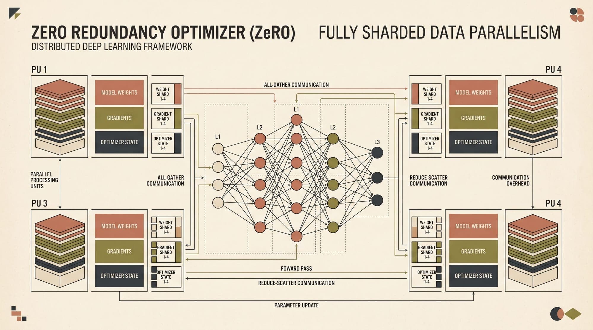
Training modern frontier large language models requires orchestrating compute across thousands of accelerators. As parameter counts scaled from billions to hundreds of billions, the memory capacity of single accelerators (such as 80 GB on an NVIDIA H100 or 96 GB on an H200) became a primary scaling bottleneck. Traditional distributed training paradigms relied on standard Data Parallelism (DDP), where every GPU maintains a complete replica of the model weights, gradients, and optimizer states, synchronizing only gradients during the backward pass via all-reduce collectives.

Under standard DDP, the memory required to store static training states scales linearly with parameter count and does not decrease as more GPUs are added. This memory wall motivated the development of memory-partitioned data-parallel paradigms: the Zero Redundancy Optimizer (ZeRO), introduced by Rajbhandari et al. (2019) at Microsoft Research, and Fully Sharded Data Parallelism (FSDP), formalized by Zhao et al. (2023) at Meta.

ZeRO and FSDP eliminate memory redundancies by sharding optimizer states, gradients, and model parameters across data-parallel ranks, reconstructing full layers dynamically on-demand during forward and backward computations through collective communication primitives.

The Memory Footprint of Large Language Model Training

To analyze why memory partitioning is necessary, consider the static and dynamic memory consumption of training an autoregressive Transformer containing $\Phi$ parameters using mixed-precision arithmetic (FP16 or BF16 forward/backward passes with 32-bit floating-point master weights and optimizer states).

Static Memory Allocation: Parameters, Gradients, and Optimizer States

In mixed-precision training with the standard AdamW optimizer, memory is divided into three primary categories:

1. Model Parameters ($M_p$): Parameters are stored in 16-bit half-precision (FP16 or BF16) for matrix multiplications in forward and backward passes.

$$M_p = 2\Phi \text{ bytes}$$

1. Gradients ($M_g$): Gradients computed during backpropagation are stored in 16-bit precision.

$$M_g = 2\Phi \text{ bytes}$$

1. Optimizer States ($M_{opt}$): To ensure numerical stability in weight updates, AdamW tracks higher-precision internal states:

• FP32 master weights: $4\Phi$ bytes
• FP32 first momentum vector ($m_t$): $4\Phi$ bytes
• FP32 second uncentered variance vector ($v_t$): $4\Phi$ bytes

$$M_{opt} = 4\Phi + 4\Phi + 4\Phi = 12\Phi \text{ bytes}$$

Summing these components yields the total static memory per parameter:

$$M_{static} = M_p + M_g + M_{opt} = 2\Phi + 2\Phi + 12\Phi = 16\Phi \text{ bytes}$$

When systems maintain FP32 gradient buffers during optimizer step reduction, this footprint expands to $18\Phi$ bytes.

+----------------------------------------------------------------------------------+
| Standard Data Parallelism (DDP) Memory per GPU (Total: 16Φ Bytes)                 |
+----------------------------------------------------------------------------------+
| Parameters (FP16/BF16) : 2Φ Bytes  [==================]                          |
| Gradients  (FP16/BF16) : 2Φ Bytes  [==================]                          |
| Master Weights (FP32)  : 4Φ Bytes  [====================================]        |
| Momentum m_t   (FP32)  : 4Φ Bytes  [====================================]        |
| Variance v_t   (FP32)  : 4Φ Bytes  [====================================]        |
+----------------------------------------------------------------------------------+

For a 70-billion parameter model ($\Phi = 70 \times 10^9$):

• Static memory requirement: $16 \times 70 \times 10^9 \text{ bytes} \approx 1,120 \text{ GB}$.
• On an 80 GB GPU, standard DDP cannot fit even the static model state of a 5-billion parameter model once activation buffers are accounted for ($16 \times 5 = 80 \text{ GB}$).

Dynamic Memory Allocation: Activations, Temporary Buffers, and Fragmentation

Beyond static states, training consumes dynamic memory:

• Activation Memory: Intermediate tensors stored during the forward pass for gradient computation during the backward pass. For a Transformer layer with hidden dimension $h$, sequence length $s$, batch size $b$, and attention heads $a$, activation memory scales as $\mathcal{O}(b \cdot s \cdot h \cdot L)$, where $L$ is layer depth. Activation checkpointing (Chen et al., 2016) trades recomputation compute for memory reduction.
• Temporary Buffers: Communication buffers for tensor coalescing, fused kernel workspaces, and PyTorch CUDA allocator memory fragmentation.

<img src="https://cms.llms.blog/content/images/2026/08/zero-memory-partitioning.png" alt="Memory Partitioning Stages across ZeRO and FSDP" />

Mathematical Formulation of ZeRO Partitioning Stages

ZeRO addresses memory redundancy by partitioning states across $N_d$ data-parallel devices while maintaining the exact algorithmic semantics of standard data-parallel training.

ZeRO-Stage 1: Optimizer State Partitioning ($P_{os}$)

In ZeRO-Stage 1 ($P_{os}$), model parameters and gradients remain fully replicated on every device, but the $12\Phi$ bytes of AdamW optimizer states are partitioned equally across all $N_d$ data-parallel ranks.

Each GPU $i \in \{1, \dots, N_d\}$ manages an optimizer state slice of size $\frac{\Phi}{N_d}$. The static memory footprint per GPU becomes:

$$M(\text{ZeRO-1}) = 2\Phi + 2\Phi + \frac{12\Phi}{N_d} = 4\Phi + \frac{12\Phi}{N_d} \text{ bytes}$$

As the data-parallel degree $N_d$ grows large:

$$\lim_{N_d \to \infty} M(\text{ZeRO-1}) = 4\Phi \text{ bytes}$$

This represents a $4\times$ memory reduction compared to standard DDP ($16\Phi \to 4\Phi$).

Execution Flow for ZeRO-1:

1. Forward and backward passes execute identically to standard DDP on full local parameters.
2. At the end of backpropagation, gradients are reduced across all $N_d$ devices using a Reduce-Scatter collective operation, such that each rank $i$ receives the averaged gradient corresponding solely to its assigned partition $\Phi_i$.
3. Rank $i$ updates its local master weights and optimizer states using the reduced gradient shard.
4. An All-Gather collective operation gathers the updated FP16/BF16 parameter shards from all ranks to reconstruct the complete parameter tensor $\Phi$ on every GPU before the next forward step.

ZeRO-Stage 2: Gradient and Optimizer State Partitioning ($P_{os+g}$)

In ZeRO-Stage 2 ($P_{os+g}$), both optimizer states and gradients are partitioned across the $N_d$ ranks.

Each GPU retains only the gradient slice corresponding to its optimizer state partition. As gradients are computed layer-by-layer during backpropagation, they are immediately reduced and scattered, removing the requirement to store full $2\Phi$ gradient buffers on every device.

The memory footprint per GPU becomes:

$$M(\text{ZeRO-2}) = 2\Phi + \frac{2\Phi}{N_d} + \frac{12\Phi}{N_d} = 2\Phi + \frac{14\Phi}{N_d} \text{ bytes}$$

As $N_d$ approaches infinity:

$$\lim_{N_d \to \infty} M(\text{ZeRO-2}) = 2\Phi \text{ bytes}$$

This achieves an $8\times$ reduction in static memory relative to standard DDP.

+----------------------------------------------------------------------------------+
| Memory Partitioning Stages Comparison (N_d ranks)                                 |
+----------------------------------------------------------------------------------+
| Standard DDP :  2Φ (Params)  +  2Φ (Grads)  +  12Φ (Optimizer)  = 16Φ            |
| ZeRO-Stage 1 :  2Φ (Params)  +  2Φ (Grads)  + (12Φ / N_d)       = 4Φ + 12Φ/N_d   |
| ZeRO-Stage 2 :  2Φ (Params)  + (2Φ / N_d)   + (12Φ / N_d)       = 2Φ + 14Φ/N_d   |
| ZeRO-Stage 3 : (2Φ / N_d)    + (2Φ / N_d)   + (12Φ / N_d)       = 16Φ / N_d      |
+----------------------------------------------------------------------------------+

ZeRO-Stage 3 and Fully Sharded Data Parallelism: Parameter Partitioning ($P_{os+g+p}$)

ZeRO-Stage 3 (and PyTorch FSDP Full Shard mode) partitions all three components: model parameters, gradients, and optimizer states.

Each GPU holds only a $\frac{1}{N_d}$ fraction of the parameters, gradients, and optimizer states:

$$M(\text{ZeRO-3/FSDP}) = \frac{2\Phi}{N_d} + \frac{2\Phi}{N_d} + \frac{12\Phi}{N_d} = \frac{16\Phi}{N_d} \text{ bytes}$$

As $N_d$ increases, the static memory footprint per device scales inversely with cluster size, dropping toward zero:

$$\lim_{N_d \to \infty} M(\text{ZeRO-3}) = 0 \text{ bytes}$$

For a 70B parameter model distributed across 64 GPUs ($N_d = 64$):

• Standard DDP: $1,120 \text{ GB}$ per GPU (infeasible).
• ZeRO-Stage 1: $280 + \frac{840}{64} = 293.1 \text{ GB}$ per GPU (infeasible for 80 GB).
• ZeRO-Stage 2: $140 + \frac{980}{64} = 155.3 \text{ GB}$ per GPU (infeasible for 80 GB).
• ZeRO-Stage 3 / FSDP: $\frac{1,120}{64} = 17.5 \text{ GB}$ per GPU (comfortably fits on an 80 GB H100 with ample headroom for activations).

Communication Complexity and Collective Primitives

A common misconception is that partitioning model states introduces severe communication overhead. The mathematical analysis of collective communication algorithms demonstrates why ZeRO-1 and ZeRO-2 impose zero communication overhead over standard DDP, and why ZeRO-3 introduces an exact 50% increase.

Standard Ring-AllReduce Communication Analysis

In standard DDP, gradient synchronization uses a Ring-AllReduce algorithm across $N$ ranks. A Ring-AllReduce of a tensor with $\Phi$ elements is executed in two consecutive phases:

1. Scatter-Reduce Phase: The ring transfers $\frac{\Phi}{N}$ data chunks across $N-1$ steps. Each rank sends and receives a total volume of:

$$V_{\text{scatter}} = \frac{N - 1}{N} \Phi \text{ elements}$$

1. All-Gather Phase: The ring gathers the accumulated values across $N-1$ steps. Each rank sends and receives:

$$V_{\text{gather}} = \frac{N - 1}{N} \Phi \text{ elements}$$

The total data sent and received per GPU during standard DDP gradient synchronization is:

$$V_{\text{DDP}} = V_{\text{scatter}} + V_{\text{gather}} = 2 \cdot \frac{N - 1}{N} \Phi \approx 2\Phi \text{ elements}$$

Standard DDP Communication:
Forward Pass  : 0 communication
Backward Pass : Ring-AllReduce(Gradients) = 2 * ((N-1)/N) * Φ
Total per Step: 2 * ((N-1)/N) * Φ

ZeRO-1 and ZeRO-2 Communication Volume

In ZeRO-1 and ZeRO-2:

1. During the backward pass, gradients are not reduced with a full All-Reduce. Instead, a Reduce-Scatter operation reduces and partitions gradients directly to the rank that owns that optimizer state shard.

$$V_{\text{Reduce-Scatter}} = \frac{N - 1}{N} \Phi \text{ elements}$$

1. Each rank computes parameter updates locally for its partition $\Phi_i$.
2. After the optimizer step, an All-Gather collective broadcasts the updated parameter shards to all ranks.

$$V_{\text{All-Gather}} = \frac{N - 1}{N} \Phi \text{ elements}$$

Total communication volume for ZeRO-1 and ZeRO-2:

$$V_{\text{ZeRO-1/2}} = V_{\text{Reduce-Scatter}} + V_{\text{All-Gather}} = 2 \cdot \frac{N - 1}{N} \Phi \approx 2\Phi \text{ elements}$$

The total communication volume of ZeRO-1 and ZeRO-2 is identical to standard DDP:

$$V_{\text{ZeRO-1/2}} = V_{\text{DDP}}$$

ZeRO-1 and ZeRO-2 achieve up to an $8\times$ reduction in static memory footprint with zero added network communication bandwidth requirement.

ZeRO-1 & ZeRO-2 Communication:
Forward Pass  : 0 communication
Backward Pass : Reduce-Scatter(Gradients) = ((N-1)/N) * Φ
Post-Step     : All-Gather(Updated Params) = ((N-1)/N) * Φ
Total per Step: 2 * ((N-1)/N) * Φ  (Exact parity with DDP)

ZeRO-3 and FSDP Communication Volume

In ZeRO-3 / FSDP, full parameters are not retained in memory. Instead, parameters are fetched dynamically before layer computation and discarded immediately after:

1. Forward Pass: Before computing layer $l$, an All-Gather reconstructs the full weights $W_l$. Once layer $l$ finishes computation, the unsharded weights are freed from memory (retaining only the local shard).

$$V_{\text{forward}} = \frac{N - 1}{N} \Phi \text{ elements}$$

1. Backward Pass (Parameters): During backpropagation, layer $l$ requires full weights $W_l$ to compute input gradients $\nabla x_l$. An All-Gather reconstructs $W_l$ a second time. Once computed, the full weights are freed.

$$V_{\text{backward, params}} = \frac{N - 1}{N} \Phi \text{ elements}$$

1. Backward Pass (Gradients): Layer $l$ computes parameter gradients $\nabla W_l$. A Reduce-Scatter reduces and distributes these gradients to the respective shard owners, freeing full gradient buffers.

$$V_{\text{backward, grads}} = \frac{N - 1}{N} \Phi \text{ elements}$$

Summing these three collective operations:

$$V_{\text{ZeRO-3/FSDP}} = V_{\text{forward}} + V_{\text{backward, params}} + V_{\text{backward, grads}} = 3 \cdot \frac{N - 1}{N} \Phi \approx 3\Phi \text{ elements}$$

The communication overhead of ZeRO-3 / FSDP relative to standard DDP is:

$$\frac{V_{\text{ZeRO-3}}}{V_{\text{DDP}}} = \frac{3 \cdot \frac{N - 1}{N} \Phi}{2 \cdot \frac{N - 1}{N} \Phi} = 1.5$$

ZeRO-3 / FSDP incurs an exact 50% communication overhead over standard DDP while reducing memory footprint to $\frac{16\Phi}{N_d}$, enabling training of arbitrary model sizes across distributed nodes.

ZeRO-3 / FSDP Layer Execution Lifecycle:

Forward Pass:
  [All-Gather Weights W_l] ──> [Compute Forward: Y_l = f(X_l, W_l)] ──> [Free Unsharded W_l]

Backward Pass:
  [All-Gather Weights W_l] ──> [Compute Gradients: ∇X_l, ∇W_l] ─────> [Free Unsharded W_l]
                                       │
                                       └──> [Reduce-Scatter ∇W_l] ───> [Free Unsharded ∇W_l]

PyTorch FSDP Internal Architecture: FlatParameter vs. Per-Parameter Sharding

PyTorch's native implementation of Fully Sharded Data Parallel has evolved across two generations, reflecting practical lessons in memory management and execution scheduling.

FSDP-1: FlatParameter and Module-Level Wrapping

In the original PyTorch FSDP architecture (Zhao et al., 2023), models are partitioned by wrapping submodules (e.g. individual Transformer decoder layers) into discrete FSDP units.

Within each FSDP unit:

• All constituent parameter tensors (e.g., $W_q, W_k, W_v, W_o, W_{\text{gate}}, W_{\text{up}}, W_{\text{down}}$) are flattened into a single contiguous 1D tensor called a FlatParameter.
• The FlatParameter is padded to be divisible by the world size $N_d$ and sliced into $N_d$ equal chunks.
• During forward/backward execution, the unit triggers a single All-Gather on the contiguous FlatParameter, minimizing collective launch overhead and kernel launch latency.

import torch
import torch.nn as nn
from torch.distributed.fsdp import (
    FullyShardedDataParallel as FSDP,
    ShardingStrategy,
    MixedPrecision,
    BackwardPrefetch,
)
from torch.distributed.fsdp.wrap import transformer_auto_wrap_policy

def setup_fsdp1_model(model: nn.Module, transformer_layer_cls: type) -> FSDP:
    auto_wrap_policy = functools.partial(
        transformer_auto_wrap_policy,
        transformer_layer_cls={transformer_layer_cls},
    )
    
    mixed_precision_policy = MixedPrecision(
        param_dtype=torch.bfloat16,
        reduce_dtype=torch.bfloat16,
        buffer_dtype=torch.bfloat16,
    )
    
    fsdp_model = FSDP(
        model,
        auto_wrap_policy=auto_wrap_policy,
        sharding_strategy=ShardingStrategy.FULL_SHARD,  # ZeRO-3 equivalent
        mixed_precision=mixed_precision_policy,
        backward_prefetch=BackwardPrefetch.BACKWARD_PRE,
        device_id=torch.cuda.current_device(),
        limit_all_gathers=True,
    )
    return fsdp_model

FSDP-2: Per-Parameter Sharding via DTensor (fully_shard)

While FlatParameter offered high memory compaction, it introduced overhead: original tensor identities were obscured, parameter inspection required custom metadata lookups, and dynamically freezing parameters or running mixed-layer architectures required complex workarounds.

PyTorch 2.x introduced FSDP-2 through the torch.distributed.fsdp.fully_shard API, built on top of Distributed Tensor (DTensor). In FSDP-2:

• Tensors are sharded individually along their leading dimension without 1D flattening.
• Sharding layouts are expressed via DTensor mesh placements Shard(0) and Replicate().
• Collective communications for individual parameters within a layer are grouped using PyTorch's asynchronous CUDA streams and coalesced communication buffers.

Overlapping Computation and Communication Streams

To hide the 50% communication overhead in ZeRO-3/FSDP, distributed runtimes use dual CUDA stream execution:

1. Compute Stream: Executes CUDA matrix multiplications (GEMMs) and attention kernels for layer $l$.
2. Communication Stream: Concurrently runs the All-Gather collective for layer $l+1$ in the forward pass, or layer $l-1$ in the backward pass.

Timeline: Forward Pass Overlap

Compute Stream :  [ Compute Layer l ] ────────────> [ Compute Layer l+1 ]
                         ▲                                 ▲
                         │ (Sync)                          │ (Sync)
Communication  :  [ All-Gather Layer l+1 ] ───────> [ All-Gather Layer l+2 ]

When network bandwidth satisfies the arithmetic intensity threshold (computation time $T_{\text{comp}} \ge$ communication time $T_{\text{comm}}$), the communication overhead of parameter reconstruction is completely overlapped behind arithmetic execution.

ZeRO-Offload and ZeRO-Infinity: Tiered Memory Architectures

When model parameters exceed aggregate GPU high-bandwidth memory (HBM), ZeRO-Offload (Ren et al., 2021) and ZeRO-Infinity (Rajbhandari et al., 2021) exploit the broader host memory hierarchy: host CPU DRAM and Non-Volatile Memory (NVMe SSDs).

ZeRO-Offload Mechanics

ZeRO-Offload structures compute and data placement based on the compute-to-memory ratio of each operation:

• GPU Operations: Forward pass ($2\Phi$ FLOPs per token) and backward pass ($4\Phi$ FLOPs per token) have high computational density ($\mathcal{O}(\text{batch} \cdot \text{seq} \cdot \text{dim})$ FLOPs per parameter transferred). These execute on the GPU.
• CPU Operations: The AdamW optimizer step performs $\mathcal{O}(1)$ operations per parameter update ($m_t, v_t$ calculations). These execute on the host CPU.

ZeRO-Offload Operational Loop:

       GPU (HBM)                                         Host CPU (DRAM)
+-----------------------+                             +------------------------+
| 1. Forward Pass       |                             |                        |
| 2. Backward Pass      |                             |                        |
| 3. Compute Gradients  | ─── Transfer Gradients ───> | 4. Receive Gradients   |
|                       |      (via PCIe / CXL)       | 5. Run FP32 Adam Step  |
| 7. Receive Parameters | <── Transfer Parameters ─── | 6. Update FP32 Weights |
+-----------------------+      (via PCIe / CXL)       +------------------------+

Communication Bandwidth Limits across Memory Biers

Transferring model parameters and gradients across the host-device interface introduces a latency bottleneck governed by PCIe / CXL bandwidth:

• NVLink 4.0 / 5.0 (GPU-to-GPU): 900 GB/s to 1,800 GB/s bidirectional bandwidth.
• PCIe Gen5 x16 (Host-to-GPU): 63 GB/s bidirectional bandwidth.
• PCIe Gen4 x16 (Host-to-GPU): 31.5 GB/s bidirectional bandwidth.

To avoid PCIe transfer stalls during CPU offloading, gradient transfer from GPU to CPU is overlapped with the backward pass computation of earlier layers, and parameter transfer from CPU to GPU is overlapped with optimizer execution.

Distributed Training Paradigms: Trade-offs and 3D Parallelism

In large-scale distributed training clusters (e.g. 1,024 to 16,384 GPUs), engineering teams combine FSDP with Tensor Parallelism (TP) and Pipeline Parallelism (PP) in a 3D parallelism topology.

Trade-off Matrix

| Parallelism Strategy | Partitioned Target | Memory Saving Factor | Communication Primitive | Primary Network Domain | Scaling Limit | | :--- | :--- | :--- | :--- | :--- | :--- | | Standard DDP | None | $1\times$ | All-Reduce | Inter-node / Intra-node | Fits single GPU model size | | ZeRO-1 ($P_{os}$) | Optimizer States | Up to $4\times$ | Reduce-Scatter + All-Gather | Inter-node / Intra-node | Scalable ($0\%$ extra volume) | | ZeRO-2 ($P_{os+g}$) | Optimizer + Grads | Up to $8\times$ | Reduce-Scatter + All-Gather | Inter-node / Intra-node | Scalable ($0\%$ extra volume) | | ZeRO-3 / FSDP | Params + Grads + Opt | Proportional to $N_d$ | All-Gather (Fwd/Bwd) + Reduce-Scatter | High-bandwidth cluster | $1.5\times$ communication volume | | Tensor Parallel (TP) | Layer Matrix Slices | Proportional to $N_{tp}$ | All-Reduce (2 per layer) | Intra-node (NVLink only) | Typically $N_{tp} \le 8$ GPUs | | Pipeline Parallel (PP) | Layer Groups | Proportional to $N_{pp}$ | Point-to-point P2P (activations) | Inter-node / Intra-node | Limited by bubble overhead |

Hybrid Sharded Data Parallelism (HSDP)

When scaling FSDP across thousands of nodes connected via slower inter-node networking (e.g., 400 Gbps InfiniBand or RoCE), running full ZeRO-3 across all nodes can saturate inter-node switches.

Hybrid Sharded Data Parallelism (HSDP) splits the data-parallel group into a 2D hierarchy:

1. Intra-node (within 8 GPUs on an NVLink switch): Full ZeRO-3 parameter sharding takes advantage of 900 GB/s NVLink bandwidth to execute fast All-Gather operations.
2. Inter-node (across server chassis): Standard DDP or ZeRO-1 optimizer sharding is applied across nodes, limiting inter-node traffic to gradient reductions at step boundaries.

HSDP 2D Communication Hierarchy:

Node 1 (8 GPUs via NVLink)                     Node 2 (8 GPUs via NVLink)
+------------------------------------+         +------------------------------------+
| GPU 0  GPU 1  GPU 2 ... GPU 7      |         | GPU 8  GPU 9  GPU 10 ... GPU 15    |
| [ Full ZeRO-3 Sharded via NVLink ] |         | [ Full ZeRO-3 Sharded via NVLink ] |
+------------------------------------+         +------------------------------------+
                  ▲                                              ▲
                  │                                              │
                  └────────── Inter-Node Network ────────────────┘
                       (ZeRO-1 / DDP Gradient Sync)

Summary of Core Principles

1. Static Memory Footprint: Standard mixed-precision training requires $16\Phi$ bytes per parameter ($2\Phi$ parameters, $2\Phi$ gradients, $12\Phi$ AdamW optimizer states).
2. Zero-Overhead Memory Reduction: ZeRO-1 and ZeRO-2 reduce static memory by $4\times$ to $8\times$ without increasing communication volume beyond standard DDP's $2 \cdot \frac{N-1}{N} \Phi$ elements.
3. Linear Parameter Scaling: ZeRO-3 and FSDP partition all static states, reducing per-GPU memory to $\frac{16\Phi}{N_d}$ bytes at the expense of a fixed 50% communication volume increase ($3 \cdot \frac{N-1}{N} \Phi$ elements).
4. Communication Overlap: Dual CUDA streams enable asynchronous prefetching of next-layer weights during current-layer computation, hiding communication latency behind compute kernels.
5. Hierarchical Topology: Combining intra-node ZeRO-3 with inter-node ZeRO-1 (HSDP) matches distributed communication patterns to the physical bandwidth hierarchy of modern AI clusters.

Sources

• Rajbhandari, S., Rasley, J., Ruwase, O., & He, Y. (2019). ZeRO: Memory Optimizations Toward Training Trillion Parameter Models. arXiv:1910.02054.
• Zhao, Y., Gu, A., Varma, R., Luo, L., Huang, C. C., Xu, M., Wright, L., Shojanazeri, H., Ott, M., Shleifer, S., Desmaison, A., Balioglu, C., Damania, P., Nguyen, B., Hao, Y., & Li, S. (2023). PyTorch FSDP: Experiences on Scaling Fully Sharded Data Parallel. arXiv:2304.11277.
• Ren, J., Rajbhandari, S., Aminabadi, R. Y., Ruwase, O., Zheng, S., Lin, E. Z., Zhang, Z., & He, Y. (2021). ZeRO-Offload: Democratizing Billion-Scale Model Training. arXiv:2101.06840.
• Rajbhandari, S., Ruwase, O., Rasley, J., Zhang, S., & He, Y. (2021). ZeRO-Infinity: Breaking the GPU Memory Wall for Extreme Scale Deep Learning. arXiv:2104.07829.
• Shoeybi, M., Patwary, M., Puri, R., LeGresley, P., Casper, J., & Catanzaro, B. (2019). Megatron-LM: Training Multi-Billion Parameter Language Models Using Model Parallelism. arXiv:1909.08053.
• Chen, T., Xu, B., Zhang, C., & Guestrin, C. (2016). Training Deep Nets with Sublinear Memory Cost. arXiv:1604.06174.
• Ba, J. L., Kiros, J. R., & Hinton, G. E. (2016). Layer Normalization. arXiv:1607.06450.