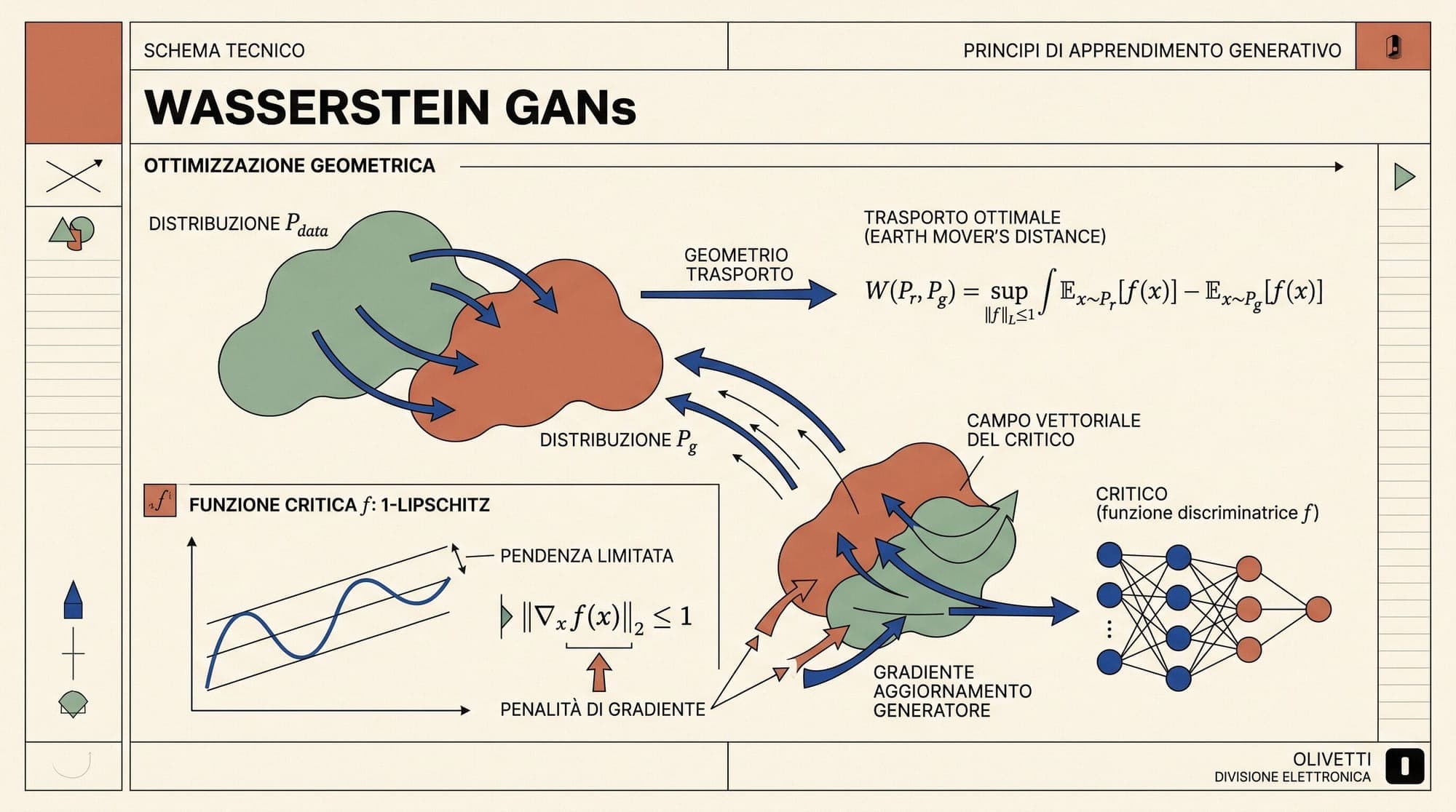
Wasserstein GANs: How Earth Mover's Distance, Kantorovich-Rubinstein Duality, and Gradient Penalties Fixed Generative Adversarial Training

Generative Adversarial Networks (Goodfellow et al., 2014) established an influential paradigm for generative modeling: formulating data synthesis as a minimax game between a generator mapping latent noise to data space and a discriminator distinguishing synthetic samples from real empirical data. Despite early empirical success, the original GAN formulation suffered from chronic training instabilities, vanishing gradients, hyperparameter fragility, and catastrophic mode collapse.

The mathematical diagnosis for these failures was established by Arjovsky and Bottou (2017): the classical GAN objective implicitly optimizes the Jensen-Shannon divergence (JSD) between the true data distribution and the model distribution. In high-dimensional spaces where distributions reside on lower-dimensional submanifolds, JSD is discontinuous and locally constant almost everywhere, yielding zero gradient information to the generator.

The introduction of the Wasserstein GAN (Arjovsky, Chintala, and Bottou, 2017) and its gradient-penalized variant WGAN-GP (Gulrajani et al., 2017) resolved these structural pathologies by replacing statistical divergences with the Earth Mover's (Wasserstein-1) distance. By leveraging the Kantorovich-Rubinstein duality theorem and enforcing 1-Lipschitz continuity on the critic network, WGAN provided continuous, non-vanishing gradients across disjoint supports and established the first generative training loss that quantitatively correlates with sample fidelity.

1. The Pathology of Classical GAN Objectives

In the vanilla formulation of Goodfellow et al. (2014), the generator transforms prior noise into synthetic samples, while the discriminator outputs the probability that a given sample is drawn from the empirical data distribution. The minimax objective is defined as:

$$\min_G \max_D V(D, G) = \mathbb{E}_{x \sim \mathbb{P}_r}[\log D(x)] + \mathbb{E}_{z \sim p(z)}[\log(1 - D(G(z)))]$$

For a fixed generator, the optimal discriminator can be computed analytically by differentiating the objective with respect to the discriminator's output:

$$D^*(x) = \frac{p_r(x)}{p_r(x) + p_g(x)}$$

Substituting the optimal discriminator back into the objective transforms the generator's optimization problem into a function of the Jensen-Shannon divergence:

$$V(D^*, G_\theta) = -\log(4) + 2 \cdot D_{JS}(\mathbb{P}_r \parallel \mathbb{P}_\theta)$$

where the Jensen-Shannon divergence is the symmetrized Kullback-Leibler (KL) divergence to the mixture distribution:

$$D_{JS}(\mathbb{P}_r \parallel \mathbb{P}_\theta) = \frac{1}{2} D_{KL}\left(\mathbb{P}_r \parallel \frac{\mathbb{P}_r + \mathbb{P}_\theta}{2}\right) + \frac{1}{2} D_{KL}\left(\mathbb{P}_\theta \parallel \frac{\mathbb{P}_r + \mathbb{P}_\theta}{2}\right)$$

The Manifold Hypothesis and Dimensionality Mismatch

The fundamental flaw of optimizing the Jensen-Shannon divergence stems from the geometric structure of high-dimensional data. Real-world data distributions (such as natural images or token sequences) are supported on low-dimensional submanifolds embedded in high-dimensional ambient space. Similarly, the generator distribution is the push-forward measure of a lower-dimensional latent space, restricting generated samples to a low-dimensional manifold.

When two low-dimensional manifolds in high-dimensional space are not perfectly aligned, their intersection has measure zero with probability 1. Under these conditions:

• Disjoint Supports: The true distribution and generator distribution have disjoint supports with probability 1.
• Divergence Saturation: The KL divergence diverges to infinity, and the Jensen-Shannon divergence collapses to a saturated constant value of $\log(2)$.
• Vanishing Gradients: Because the Jensen-Shannon divergence is locally constant everywhere except on the exact data manifold, the gradient of the generator loss vanishes identically: $\nabla_\theta D_{JS}(\mathbb{P}_r \parallel \mathbb{P}_\theta) = 0$.
• Mode Collapse Under Heuristic Objectives: To prevent vanishing gradients, practitioners introduced the non-saturating objective $-\log D(G(z))$. However, as proven in Arjovsky and Bottou (2017), this objective minimizes $D_{KL}(\mathbb{P}_\theta \parallel \mathbb{P}_r) - 2 D_{JS}(\mathbb{P}_r \parallel \mathbb{P}_\theta)$, heavily penalizing improbable outputs while assigning zero penalty to dropping major modes of the target distribution.

Vanilla GAN Optimization Pathology:
Disjoint Manifolds  ──>  Optimal Discriminator D*(x) separates perfectly
                    ──>  D_JS(P_r || P_θ) = log(2) (flat plateau)
                    ──>  ∇_θ Loss = 0 (Vanishing Gradients)
Non-Saturating Loss ──>  -log D(G(z)) creates unstable gradients
                    ──>  Generator exploits single mode (Mode Collapse)

2. The Wasserstein-1 (Earth Mover's) Distance

To guarantee continuous, informative gradients throughout parameter space, the optimization metric must account for the geometric distance between points in the ambient space. The Wasserstein-1 distance arises from the theory of Optimal Transport (Villani, 2008):

$$\mathcal{W}_1(\mathbb{P}_r, \mathbb{P}_\theta) = \inf_{\gamma \in \Pi(\mathbb{P}_r, \mathbb{P}_\theta)} \mathbb{E}_{(x, y) \sim \gamma}\left[ \|x - y\| \right]$$

where $\Pi(\mathbb{P}_r, \mathbb{P}_\theta)$ denotes the set of all joint probability distributions (couplings) whose marginals satisfy the empirical data distribution and the model distribution.

Intuitively, a coupling represents a transportation plan describing how much probability mass moves from point $x$ to point $y$, while $\|x - y\|$ represents the Euclidean transport cost. The Wasserstein-1 distance identifies the optimal coupling that minimizes total expected transport work.

Metric Behavior on Disjoint Manifolds

The decisive mathematical property of the Wasserstein distance is that it metrizes a weak topology. Consider the canonical parallel line example introduced in Arjovsky et al. (2017), where distribution $P_0$ is uniform on $(0, y)$ and distribution $P_\theta$ is uniform on $(\theta, y)$ for $y \in [0, 1]$:

• Total Variation Distance: $\delta(P_0, P_\theta) = 1$ for all $\theta \neq 0$. The metric is discontinuous at $\theta = 0$, yielding $\nabla_\theta \delta = 0$.
• Kullback-Leibler Divergence: $D_{KL}(P_0 \parallel P_\theta) = +\infty$ for all $\theta \neq 0$, rendering gradients undefined.
• Jensen-Shannon Divergence: $D_{JS}(P_0 \parallel P_\theta) = \log(2)$ for all $\theta \neq 0$. The metric forms a flat plateau with $\nabla_\theta D_{JS} = 0$.
• Wasserstein-1 Distance: $\mathcal{W}_1(P_0, P_\theta) = |\theta|$. The metric is continuous and differentiable everywhere on $\mathbb{R} \setminus \{0\}$, providing a constant unit gradient $\nabla_\theta \mathcal{W}_1 = \text{sign}(\theta)$ that directs the generator straight toward $\theta = 0$.

3. The Kantorovich-Rubinstein Duality

Computing the infimum over all joint couplings is computationally intractable for continuous neural distributions. However, the Kantorovich-Rubinstein duality theorem reformulates the primal optimal transport problem into an unconstrained functional supremum:

$$\mathcal{W}_1(\mathbb{P}_r, \mathbb{P}_\theta) = \sup_{\|f\|_L \le 1} \left( \mathbb{E}_{x \sim \mathbb{P}_r}[f(x)] - \mathbb{E}_{y \sim \mathbb{P}_\theta}[f(y)] \right)$$

where $\|f\|_L \le 1$ denotes the family of 1-Lipschitz continuous functions satisfying:

$$|f(x_1) - f(x_2)| \le \|x_1 - x_2\|_2 \quad \forall x_1, x_2 \in \mathcal{X}$$

From Discriminator to Critic

Under the dual formulation, the binary classification discriminator is replaced by a scalar valuation network $f_w: \mathcal{X} \to \mathbb{R}$, termed the critic. The critic does not output probabilities or apply sigmoid activations. Instead, it outputs unbounded real scalar potentials representing the cost landscape of optimal transport.

When parameterized by weights $w$ under the 1-Lipschitz constraint, the critic objective is:

$$\max_{w, \|f_w\|_L \le 1} \mathbb{E}_{x \sim \mathbb{P}_r}[f_w(x)] - \mathbb{E}_{z \sim p(z)}[f_w(G_\theta(z))]$$

When the critic is optimized to approximate the supremum $f^*$, the gradient of the Wasserstein distance with respect to generator parameters $\theta$ is differentiable almost everywhere (Arjovsky et al., 2017):

$$\nabla_\theta \mathcal{W}_1(\mathbb{P}_r, \mathbb{P}_\theta) = -\mathbb{E}_{z \sim p(z)}\left[ \left.\nabla_x f^*(x)\right|_{x = G_\theta(z)} \cdot \nabla_\theta G_\theta(z) \right]$$

This result demonstrates that the generator can be trained via standard backpropagation directly through the critic's spatial gradient field.

4. Enforcing 1-Lipschitz Continuity

Enforcing the 1-Lipschitz constraint on deep neural networks represents the primary operational challenge in Wasserstein GAN architectures.

4.1 Weight Clipping (Original WGAN)

In the initial WGAN formulation (Arjovsky et al., 2017), the authors enforced Lipschitz bounds by clamping all network parameters to a fixed interval $[-c, c]$ after each optimization step:

$$w \leftarrow \text{clip}(w, -c, c)$$

Because compositions of linear transformations with bounded weights and 1-Lipschitz activations (such as ReLU or LeakyReLU) are Lipschitz continuous, weight clipping satisfies the condition up to a scaling constant.

However, weight clipping introduces severe failure modes:

• Capacity Saturation: Gradient ascent drives the critic weights toward the extreme values $+c$ and $-c$. As documented in Gulrajani et al. (2017), this restricts the network to excessively simple, piecewise linear functions.
• Vanishing and Exploding Gradients: The effective Lipschitz constant scales exponentially with network depth ($c^L$). Minor miscalibrations of $c$ cause vanishing gradients when $c$ is too small or exploding gradients when $c$ is too large.

4.2 Gradient Penalty (WGAN-GP)

To eliminate the pathologies of weight clipping, Gulrajani et al. (2017) introduced the Gradient Penalty formulation (WGAN-GP).

By Rademacher's theorem, a differentiable function $f$ is 1-Lipschitz if and only if its gradient norm satisfies $\|\nabla_x f(x)\|_2 \le 1$ almost everywhere. Under optimal transport theory, the optimal critic function $f^*$ attains unit gradient norm almost everywhere along straight lines connecting real and generated samples:

$$\|\nabla_{\hat{x}} f^*(\hat{x})\|_2 = 1$$

WGAN-GP enforces this condition by sampling random convex combinations of real and generated instances:

$$\hat{x} = \epsilon x + (1 - \epsilon)\tilde{x} \quad \text{where } \epsilon \sim U[0, 1], \quad x \sim \mathbb{P}_r, \quad \tilde{x} \sim \mathbb{P}_\theta$$

and penalizing deviations from unit gradient norm. The complete WGAN-GP critic loss is:

$$\mathcal{L}_{critic} = \mathbb{E}_{\tilde{x} \sim \mathbb{P}_\theta}[f_w(\tilde{x})] - \mathbb{E}_{x \sim \mathbb{P}_r}[f_w(x)] + \lambda \mathbb{E}_{\hat{x} \sim \mathbb{P}_{\hat{x}}}\left[ \left( \|\nabla_{\hat{x}} f_w(\hat{x})\|_2 - 1 \right)^2 \right]$$

where $\lambda = 10$ provides stable optimization across vision, audio, and language representations.

Incompatibility with Batch Normalization

Gradient penalties require evaluating $\|\nabla_{\hat{x}} f_w(\hat{x})\|_2$ with respect to individual samples independently. Batch Normalization introduces inter-sample statistical dependencies across the minibatch, which invalidates single-instance gradient norm calculations and causes optimization failure. WGAN-GP architectures must replace Batch Normalization in the critic with Layer Normalization, Instance Normalization, or Group Normalization.

4.3 Spectral Normalization (SNGAN)

An alternative formulation by Miyato et al. (2018) constrains the Lipschitz constant by normalizing the spectral norm (matrix 2-norm) of each layer's weight matrix $W$:

$$\tilde{W}_{SN} = \frac{W}{\sigma(W)}$$

where $\sigma(W) = \max_{h \neq 0} \frac{\|Wh\|_2}{\|h\|_2}$ is the largest singular value of $W$. By ensuring that every linear layer satisfies $\|\tilde{W}_{SN}\|_2 = 1$, the composition of layers guarantees that the entire network is 1-Lipschitz without calculating explicit gradient penalties. Spectral norm estimation is computed efficiently via one step of power iteration per training batch:

$$\tilde{v} \leftarrow \frac{W^T u}{\|W^T u\|_2}, \quad \tilde{u} \leftarrow \frac{W \tilde{v}}{\|W \tilde{v}\|_2}, \quad \sigma(W) \approx u^T W v$$

5. Architectural Comparison and Training Dynamics

The structural shifts across generative adversarial paradigms illustrate how Wasserstein formulations resolved early training instabilities:

• Statistical Divergence: Standard GANs optimize Jensen-Shannon divergence; WGAN, WGAN-GP, and SNGAN optimize the continuous Earth Mover's distance.
• Output Layer: Standard GANs output probabilities via sigmoid units; Wasserstein critics output unbounded real scalar scores.
• Lipschitz Enforcement: Standard GANs apply no Lipschitz regularization; WGAN uses weight clipping; WGAN-GP uses two-sided gradient penalty; SNGAN uses spectral normalization.
• Loss Interpretability: Standard GAN discriminator loss oscillates without indicating sample quality; WGAN-GP critic loss monotonically tracks Wasserstein distance and sample fidelity.
• Normalization Strategy: Standard GANs use Batch Normalization; WGAN-GP requires LayerNorm or GroupNorm to avoid minibatch gradient coupling.
• Optimizer Configurations: Standard GANs require careful Adam momentum tuning; WGAN-GP runs reliably with Adam ($\beta_1 = 0.0, \beta_2 = 0.9$); original WGAN uses RMSProp.
• Update Schedule: Wasserstein architectures perform asymmetric training with $n_{critic} = 5$ critic steps per generator step to ensure the critic stays close to the optimal potential $f^*$.

Critic Loss as a Quantitative Quality Metric

In classical GANs, discriminator loss cannot be used to monitor training progress: a low discriminator loss indicates generator failure, while high loss provides no guarantee of sample realism.

In WGAN-GP, the negative critic loss directly estimates $\mathcal{W}_1(\mathbb{P}_r, \mathbb{P}_\theta)$. As the generator converges toward the empirical distribution, $\mathcal{W}_1 \to 0$ monotonically. This correlation enables automated hyperparameter tuning and early stopping without requiring frequent evaluation of external metrics like Fréchet Inception Distance (FID).

6. PyTorch Implementation: WGAN-GP Training Step

The following implementation details the exact gradient penalty computation and dual optimization step in PyTorch:

import torch
import torch.nn as nn
import torch.autograd as autograd

def compute_gradient_penalty(
    critic: nn.Module,
    real_samples: torch.Tensor,
    fake_samples: torch.Tensor,
    device: torch.device
) -> torch.Tensor:
    """
    Computes the two-sided gradient penalty: E[(||∇_x̂ f(x̂)||_2 - 1)^2]
    along random linear interpolations between real and generated batches.
    """
    batch_size = real_samples.size(0)
    
    # 1. Sample uniform interpolation factor ε ~ U[0, 1]
    epsilon = torch.rand(batch_size, 1, 1, 1, device=device).expand_as(real_samples)
    
    # 2. Linear interpolation: x̂ = ε * x_real + (1 - ε) * x_fake
    interpolated = (epsilon * real_samples + (1.0 - epsilon) * fake_samples).requires_grad_(True)
    
    # 3. Forward pass through critic
    critic_interpolated = critic(interpolated)
    
    # 4. Compute gradients of critic outputs with respect to interpolated inputs
    grad_outputs = torch.ones_like(critic_interpolated, device=device, requires_grad=False)
    gradients = autograd.grad(
        outputs=critic_interpolated,
        inputs=interpolated,
        grad_outputs=grad_outputs,
        create_graph=True,   # Enables backpropagation through the gradient penalty
        retain_graph=True,
        only_inputs=True,
    )[0]
    
    # 5. Flatten gradients across spatial dimensions and calculate L2 norm
    gradients = gradients.view(batch_size, -1)
    gradient_norm = gradients.norm(2, dim=1)
    
    # 6. Two-sided unit norm penalty
    gradient_penalty = torch.mean((gradient_norm - 1.0) ** 2)
    return gradient_penalty

def train_wgan_gp_step(
    generator: nn.Module,
    critic: nn.Module,
    opt_gen: torch.optim.Optimizer,
    opt_critic: torch.optim.Optimizer,
    real_images: torch.Tensor,
    latent_dim: int,
    lambda_gp: float = 10.0,
    device: torch.device = torch.device("cuda" if torch.cuda.is_available() else "cpu")
) -> dict:
    batch_size = real_images.size(0)
    
    # -------------------------------------------------------------
    # Critic Update (typically executed n_critic = 5 times per gen step)
    # -------------------------------------------------------------
    opt_critic.zero_grad()
    
    z = torch.randn(batch_size, latent_dim, device=device)
    fake_images = generator(z).detach()
    
    critic_real = critic(real_images)
    critic_fake = critic(fake_images)
    
    gp = compute_gradient_penalty(critic, real_images, fake_images, device)
    critic_loss = torch.mean(critic_fake) - torch.mean(critic_real) + lambda_gp * gp
    
    critic_loss.backward()
    opt_critic.step()
    
    wasserstein_estimate = (torch.mean(critic_real) - torch.mean(critic_fake)).item()
    
    # -------------------------------------------------------------
    # Generator Update
    # -------------------------------------------------------------
    opt_gen.zero_grad()
    gen_z = torch.randn(batch_size, latent_dim, device=device)
    gen_fake_images = generator(gen_z)
    
    # Generator maximizes critic potential: min -E[f(G(z))]
    gen_loss = -torch.mean(critic(gen_fake_images))
    gen_loss.backward()
    opt_gen.step()
    
    return {
        "critic_loss": critic_loss.item(),
        "gen_loss": gen_loss.item(),
        "wasserstein_distance": wasserstein_estimate,
        "gradient_penalty": gp.item()
    }

7. Modern Legacy in Diffusion and Flow Matching

The mathematical insights established by Wasserstein GANs laid the theoretical foundation for contemporary generative architectures:

1. Optimal Transport Flow Matching (OT-CFM): Modern continuous normalizing flows (Lipman et al., 2022; Liu et al., 2022) construct probability trajectories using optimal transport displacement paths. By replacing curved stochastic trajectories with straight, constant-velocity lines between noise and data, OT-CFM enables deterministic sampling in $N \approx 4\text{--}10$ steps.
2. Score-Based Diffusion Geodesics: The critic spatial gradient $\nabla_x f^*(x)$ in WGAN represents an optimal transport displacement vector directing synthetic samples toward data probability mass, directly anticipating the score function $\nabla_x \log p(x)$ in score-based diffusion models (Song and Ermon, 2019).
3. Representation Geometry and Distribution Alignment: Kantorovich-Rubinstein duality remains the standard analytical tool for bounding representation drift, evaluating cross-modal alignment, and computing geometry-aware loss functions across large-scale vision and language models.

Sources

• Arjovsky, M., & Bottou, L. (2017). Towards Principled Methods for Training Generative Adversarial Networks. arXiv:1701.04862.
• Arjovsky, M., Chintala, S., & Bottou, L. (2017). Wasserstein Generative Adversarial Networks. International Conference on Machine Learning (ICML). arXiv:1701.07875.
• Goodfellow, I., et al. (2014). Generative Adversarial Networks. Advances in Neural Information Processing Systems (NeurIPS). arXiv:1406.2661.
• Gulrajani, I., Ahmed, F., Arjovsky, M., Dumoulin, V., & Courville, A. (2017). Improved Training of Wasserstein GANs. Advances in Neural Information Processing Systems (NeurIPS). arXiv:1704.00028.
• Lipman, Y., Chen, R. T. Q., Ben-Hamu, H., Nicklas, M., & Le, M. (2022). Flow Matching for Generative Modeling. arXiv:2210.02747.
• Liu, X., Gong, C., & Liu, Q. (2022). Flow Straight and Fast: Learning to Generate and Transfer Data with Rectified Flow. arXiv:2209.03003.
• Miyato, T., Kataoka, T., Koyama, M., & Yoshida, Y. (2018). Spectral Normalization for Generative Adversarial Networks. International Conference on Learning Representations (ICLR). arXiv:1802.05957.
• Song, Y., & Ermon, S. (2019). Generative Modeling by Estimating Gradients of the Data Distribution. NeurIPS. arXiv:1907.05600.
• Villani, C. (2008). Optimal Transport: Old and New. Springer Grundlehren der mathematischen Wissenschaften, Vol. 338.