Tensor Parallelism and Pipeline Parallelism: Mathematical Foundations of Megatron-LM 1D Slicing, Sequence Parallelism, and 1F1B Scheduling

Scaling modern large language models beyond tens of billions of parameters quickly exhausts the physical memory and compute throughput of individual graphics processing units. A 70-billion-parameter model stored in 16-bit floating-point (FP16 or BF16) requires 140 GB of VRAM solely for model weights. During full-precision training with the Adam optimizer, parameter states, gradients, and optimizer momentum terms demand approximately 16 to 18 bytes per parameter (amounting to 1.12 TB to 1.26 TB for a 70B checkpoint), completely detached from the dynamic memory required to store forward-pass activation tensors.

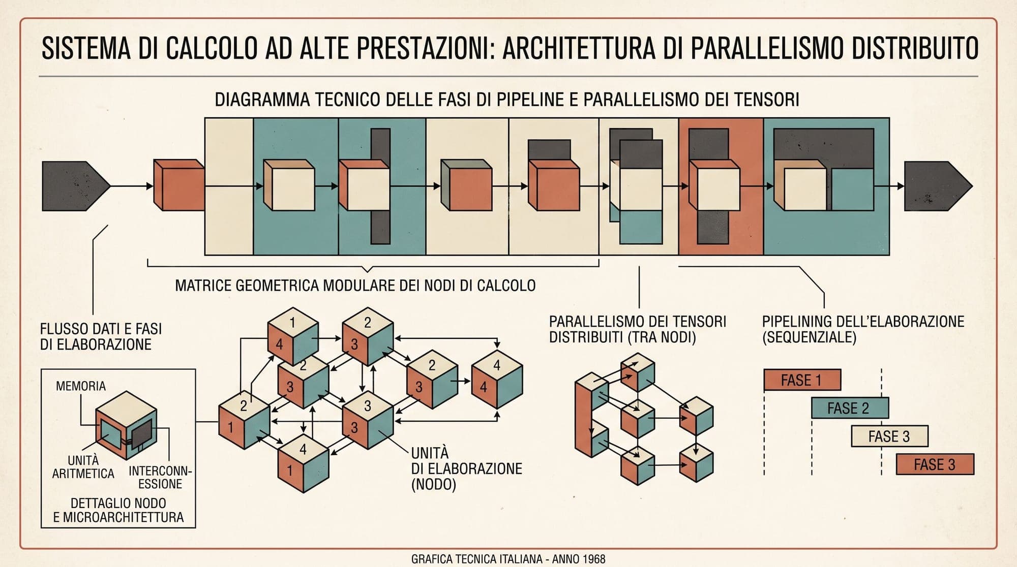
When model weights cannot fit onto a single accelerator, practitioners rely on multi-dimensional distributed parallelism. Tensor Parallelism (TP) shards individual weight matrices within each transformer layer across multiple GPUs connected via high-bandwidth interconnects. Pipeline Parallelism (PP) partitions layers sequentially across devices along the network depth.

Understanding the mathematical decomposition of matrix multiplications, the communication algebra of conjugate operators, Sequence Parallelism extensions, and the scheduling dynamics of 1F1B pipeline execution is essential for designing distributed training and inference architectures.

The Memory Footprint of Distributed Transformer Training

To understand why multi-dimensional parallelism is necessary, consider the exact memory breakdown of training a transformer parameterized by $\Phi$ weights with hidden dimension $h$, sequence length $s$, batch size $b$, and layer count $L$.

Static Memory: Weights, Gradients, and Optimizer States

In mixed-precision training using standard 32-bit Adam optimization:

• Model Weights (FP16/BF16): 2 bytes per parameter ($2\Phi$).
• Gradients (FP16/BF16): 2 bytes per parameter ($2\Phi$).
• Master Weights (FP32): 4 bytes per parameter ($4\Phi$).
• First Momentum Vector (FP32): 4 bytes per parameter ($4\Phi$).
• Second Momentum Vector (FP32): 4 bytes per parameter ($4\Phi$).

The baseline static memory footprint per parameter is:

$$M_{\text{static}} = 2\Phi + 2\Phi + 4\Phi + 4\Phi + 4\Phi = 16\Phi \text{ bytes}$$

For a model with $\Phi = 70 \times 10^9$ parameters, $M_{\text{static}} = 1.12 \text{ TB}$. On standard 80 GB NVIDIA H100 GPUs, static states alone require a minimum of 14 GPUs without accounting for intermediate activations, workspace buffers, or memory fragmentation.

Dynamic Memory: Activation Scaling

Activation memory stores the intermediate tensors produced during the forward pass that are retained for gradient computation during backpropagation. For a standard transformer layer with multi-head attention and a 4-multiple feed-forward network (FFN), the activation memory per layer $M_{\text{act}}$ scales linearly with sequence length $s$, batch size $b$, and hidden dimension $h$:

$$M_{\text{act}} = s \cdot b \cdot h \cdot \left(34 + 5 \cdot \frac{a \cdot s}{h}\right) \text{ bytes}$$

where $a$ is the number of attention heads. As sequence lengths expand to 32,768 or 128,000 tokens, activation memory exceeds static weight memory by multiples.

Megatron-LM 1D Tensor Parallelism

Introduced by Shoeybi et al. (2019) at NVIDIA, 1D Tensor Parallelism splits the linear projection matrices of Multi-Head Self-Attention (MHA) and Multi-Layer Perceptron (MLP) blocks across $t$ parallel processing units while minimizing inter-device synchronization.

Column-Parallel Linear Layer

Consider a linear transformation $Y = X A$, where $X \in \mathbb{R}^{B \times H_{\text{in}}}$ represents input activations and $A \in \mathbb{R}^{H_{\text{in}} \times H_{\text{out}}}$ is the weight matrix. In column-parallel linear layers, the weight matrix $A$ is sliced along its column dimension across $t$ GPUs:

$$A = \begin{bmatrix} A_1 & A_2 & \dots & A_t \end{bmatrix}, \quad A_i \in \mathbb{R}^{H_{\text{in}} \times \frac{H_{\text{out}}}{t}}$$

Each GPU holds the full input tensor $X$ and independently computes its local partition of the output:

$$Y_i = X A_i, \quad Y = \begin{bmatrix} Y_1 & Y_2 & \dots & Y_t \end{bmatrix}$$

Because the transformation produces partitioned columns without requiring cross-partition reduction, an element-wise non-linear activation function $\sigma(\cdot)$ (such as GeLU or SwiGLU) can be applied directly to each shard locally:

$$\sigma(Y) = \begin{bmatrix} \sigma(Y_1) & \sigma(Y_2) & \dots & \sigma(Y_t) \end{bmatrix}$$

Column parallelism eliminates communication prior to or across the activation function.

Row-Parallel Linear Layer

In a row-parallel linear layer, the subsequent weight matrix $B \in \mathbb{R}^{H_{\text{out}} \times H_{\text{final}}}$ is sliced along its row dimension across $t$ GPUs:

$$B = \begin{bmatrix} B_1 \\ B_2 \\ \vdots \\ B_t \end{bmatrix}, \quad B_i \in \mathbb{R}^{\frac{H_{\text{out}}}{t} \times H_{\text{final}}}$$

Each GPU computes the matrix product of its local input partition $Y_i \in \mathbb{R}^{B \times \frac{H_{\text{out}}}{t}}$ and its local weight slice $B_i$:

$$Z_i = Y_i B_i$$

The complete mathematical output $Z$ requires summing across all local outputs:

$$Z = \sum_{i=1}^t Y_i B_i = \sum_{i=1}^t Z_i$$

This summation is performed by an $\text{All-Reduce}$ (sum) collective communication operation across the $t$ tensor parallel ranks.

Column-Parallel:  X ──┬──> [ A_1 ] ──> Y_1 ──> GeLU ──> [ B_1 ] ──┬──> [ All-Reduce Sum ] ──> Z
                      ├──> [ A_2 ] ──> Y_2 ──> GeLU ──> [ B_2 ] ──┤
                      └──> [ A_t ] ──> Y_t ──> GeLU ──> [ B_t ] ──┘
                             (Column Slicing)               (Row Slicing)

Self-Attention Layer Decomposition

In multi-head attention, the query ($W_Q$), key ($W_K$), and value ($W_V$) projection matrices are partitioned using column parallelism. The attention heads $h$ are divided uniformly across $t$ GPUs ($h/t$ heads per rank):

• Projection Phase: Each GPU computes $Q_i = X W_Q^i$, $K_i = X W_K^i$, and $V_i = X W_V^i$.
• Attention Computation: Local heads evaluate attention maps independently:

$$\text{Head}_{i, k} = \text{Softmax}\left(\frac{Q_{i, k} K_{i, k}^T}{\sqrt{d_k}}\right) V_{i, k}$$

• Output Projection: The output projection matrix $W_O$ is partitioned using row parallelism. Each GPU multiplies its concatenated local attention head outputs with $W_O^i$.
• Synchronization: A single $\text{All-Reduce}$ collective sums the outputs across all $t$ ranks before the residual connection.

Conjugate Communication Operators

Megatron-LM defines two conjugate communication primitives, $f$ and $g$, to manage forward and backward execution:

• In Column-Parallel Layers: The forward operator $f$ is an identity mapping (no-op), while the backward operator $f^*$ computes an $\text{All-Reduce}$ (sum) of the incoming gradients $\nabla_X$.
• In Row-Parallel Layers: The forward operator $g$ executes an $\text{All-Reduce}$ (sum) across output shards, while the backward operator $g^*$ is an identity mapping.

Each transformer layer contains exactly one Attention block and one MLP block, requiring:

• Forward Pass: 2 $\text{All-Reduce}$ operations.
• Backward Pass: 2 $\text{All-Reduce}$ operations.

Using a ring-based $\text{All-Reduce}$ algorithm, the communication volume per rank for a message of size $M$ elements is $2 \cdot \frac{t - 1}{t} \cdot M$. For an activation tensor of shape $(s, b, h)$, the total bytes transmitted per layer per step equals:

$$\text{Comm}_{\text{TP}} = 8 \cdot \left(\frac{t - 1}{t}\right) \cdot s \cdot b \cdot h \cdot 2 \text{ bytes}$$

Because of the high frequency of communication (two synchronizations per transformer layer), Tensor Parallelism is strictly restricted to intra-node NVLink domains ($t \le 8$), where unidirectional bandwidth exceeds 450 to 900 GB/s per GPU.

Sequence Parallelism

While 1D Tensor Parallelism shards the GEMM weights and self-attention operations across $t$ GPUs, standard TP replicates LayerNorm, Dropout, and residual connection activations across all $t$ ranks. In modern transformer architectures, these replicated activations account for up to 10 $s \cdot b \cdot h$ bytes per layer.

Korthikanti et al. (2022) introduced Sequence Parallelism (SP) in Megatron-LM to shard activations along the sequence length dimension $s$ during non-tensor-parallel operations.

Splitting All-Reduce into Reduce-Scatter and All-Gather

Operations such as LayerNorm and Dropout operate independently along the hidden dimension $h$ for each token in the sequence. By partitioning the sequence length $s$ into $t$ chunks of size $s/t$, each GPU processes only $s/t$ tokens during LayerNorm and Dropout.

Sequence Parallelism replaces the standard $\text{All-Reduce}$ communication operators with $\text{Reduce-Scatter}$ and $\text{All-Gather}$ pairs:

1. Row-Parallel Exit: The row-parallel GEMM produces local partial sums of size $(s, b, h)$. Instead of performing an $\text{All-Reduce}$ to create a replicated full tensor, the runtime executes a $\text{Reduce-Scatter}$ operation. This simultaneously sums the partial products and shards the result along the sequence dimension, leaving each GPU with an $(s/t, b, h)$ tensor.
2. Normalized Execution: LayerNorm, residual additions, and Dropout execute locally on $(s/t, b, h)$ tensors.
3. Column-Parallel Entry: Before entering the next column-parallel GEMM (which expects the full sequence $s$ to multiply against column-sharded weights), the runtime executes an $\text{All-Gather}$ operation, reconstructing the $(s, b, h)$ activation tensor.

Mathematically, because $\text{All-Reduce} \equiv \text{Reduce-Scatter} + \text{All-Gather}$, the total communication volume of Sequence Parallelism is strictly identical to standard Tensor Parallelism:

$$\text{Volume}(\text{Reduce-Scatter}) + \text{Volume}(\text{All-Gather}) = \left(\frac{t - 1}{t} M\right) + \left(\frac{t - 1}{t} M\right) = 2 \left(\frac{t - 1}{t}\right) M = \text{Volume}(\text{All-Reduce})$$

Sequence Parallelism reduces the activation memory footprint from:

$$M_{\text{act}}^{\text{TP}} = s \cdot b \cdot h \cdot \left(10 + \frac{24}{t} + 5 \cdot \frac{a \cdot s}{h \cdot t}\right)$$

to:

$$M_{\text{act}}^{\text{TP+SP}} = \frac{s \cdot b \cdot h}{t} \cdot \left(10 + 24 + 5 \cdot \frac{a \cdot s}{h}\right)$$

Every single activation tensor in the transformer block is sharded by $1/t$ without adding network communication overhead.

Pipeline Parallelism and 1F1B Scheduling

When a model's depth exceeds what can be accommodated within a single node (even with $TP = 8$), Pipeline Parallelism (PP) partitions the $L$ layers of the network across $p$ sequential pipeline stages located on different machines.

The Pipeline Bubble in GPipe

In naive pipeline parallelism (GPipe, Huang et al., 2019), a global batch $B$ is split into $m$ microbatches ($b = B/m$). The execution flows linearly through stages $1, \dots, p$:

Stage 4:             [F1][F2][F3][F4]                 [B4][B3][B2][B1]
Stage 3:         [F1][F2][F3][F4]         [B4][B3][B2][B1]
Stage 2:     [F1][F2][F3][F4] [B4][B3][B2][B1]
Stage 1: [F1][F2][F3][F4]                 [B4][B3][B2][B1]
Time ───> | Warmup |      Steady State     | Cooldown |

During startup (warmup) and drain (cooldown), downstream and upstream devices remain idle. The fraction of execution time lost to idle hardware (the pipeline bubble fraction $F_{\text{bubble}}$) is given by:

$$F_{\text{bubble}} = \frac{p - 1}{m + p - 1}$$

When $m \gg p$, the bubble fraction approaches $(p - 1)/m$. However, in GPipe, all $m$ forward microbatches must be completed before backward passes begin, forcing stage 1 to store activations for all $m$ microbatches simultaneously:

$$M_{\text{act}}^{\text{GPipe}} = O(m) \text{ activation memory}$$

For large $m$, activation memory overwhelms physical device capacity.

1F1B (One Forward, One Backward) Schedule

To bound activation memory while maintaining pipeline throughput, Megatron-LM implements the 1F1B (One Forward, One Backward) scheduling paradigm (Narayanan et al., 2021).

In 1F1B, after a stage completes a warm-up phase of forward passes equal to its remaining downstream depth ($p - i$ microbatches for stage $i$), it enters a steady-state regime where it executes exactly one forward pass followed immediately by one backward pass for the oldest completed microbatch:

Stage 4:             [F1][B1][F2][B2][F3][B3][F4][B4]
Stage 3:         [F1][F2][B1][F3][B2][F4][B3][B4]
Stage 2:     [F1][F2][F3][B1][F4][B2][B3][B4]
Stage 1: [F1][F2][F3][F4][B1][B2][B3][B4]

Under 1F1B:

• Outstanding forward activations are retired as rapidly as they are generated.
• The maximum number of concurrently stored activation microbatches in any stage is capped at $p$, independent of total microbatch count $m$:

$$M_{\text{act}}^{\text{1F1B}} = O(p) \text{ activation memory}$$

This decoupling allows engineers to scale the number of microbatches $m$ arbitrarily high to suppress the pipeline bubble without increasing GPU memory consumption.

Interleaved 1F1B Schedule

To further minimize the bubble fraction $F_{\text{bubble}}$ without increasing batch size $m$, Megatron-LM supports interleaved virtual stages. Instead of assigning a contiguous block of $L/p$ layers to each device, each physical GPU manages $v$ virtual stages (chunks).

For example, with $p = 4$ physical GPUs and $v = 2$, GPU 1 holds Chunk 1 (Layers 1 to 2) and Chunk 5 (Layers 9 to 10). A microbatch passes through GPU 1 to GPU 2 to GPU 3 to GPU 4, then back to GPU 1 to GPU 2 to GPU 3 to GPU 4.

The resulting bubble fraction shrinks by a factor of $v$:

$$F_{\text{bubble}}^{\text{interleaved}} = \frac{p - 1}{v \cdot m}$$

The trade-off is an increase in point-to-point peer communication over the network by a factor of $v$, requiring dedicated high-speed inter-node links.

3D Parallelism Grid and Interconnect Topology

State-of-the-art frontier model training orchestrates Tensor Parallelism, Pipeline Parallelism, and Data Parallelism (DP) into a cohesive 3D grid across $N$ GPUs:

$$N = \text{TP} \times \text{PP} \times \text{DP}$$

Parallelism Dimensions Overview

• Tensor Parallelism (TP + SP): Splits intra-layer GEMMs and sequence tokens. Uses Reduce-Scatter and All-Gather collectives. Demands extremely high bandwidth (>450 GB/s) and is mapped to intra-node NVLink/NVSwitch domains.
• Pipeline Parallelism (PP): Splits model depth ($L$ layers). Uses point-to-point non-blocking send/receive operations. Requires moderate bandwidth (10 to 50 GB/s) and is mapped across inter-node InfiniBand/RoCE links.
• Data Parallelism (DP / ZeRO): Splits the batch dimension ($B$). Uses All-Reduce or Reduce-Scatter/All-Gather over parameter and gradient shards. Requires periodic bulk bandwidth (50 to 100 GB/s) across the cluster fabric.

Network Topology Mapping

Modern GPU cluster architectures (e.g., NVIDIA SuperPODs with H100/H200 nodes) feature 8 GPUs per server connected via high-bandwidth NVLink crossbar switches (900 GB/s per GPU), while inter-node communication is routed over 400 Gbps or 800 Gbps InfiniBand interfaces.

Engineers align the 3D parallelism topology directly with physical network bandwidth:

1. Set $\text{TP} \le 8$: Confine all Tensor and Sequence Parallelism communication within the intra-node NVLink domain. Crossing PCIe or InfiniBand links with Tensor Parallelism degrades arithmetic intensity and causes severe GEMM pipeline stalls.
2. Set $\text{PP} \ge 1$ across nodes: Pipeline Parallelism only transmits boundary layer activation tensors of shape $(s, b, h)$ between adjacent stages, incurring minimal point-to-point network traffic.
3. Set $\text{DP} / \text{ZeRO}$ across the remaining cluster: Data Parallelism distributes the outer batch dimension across nodes, overlapping gradient synchronization collectives with backward compute passes.

By decomposing dense matrix projections, sharding non-GEMM activations across sequence dimensions, and interleaving microbatch schedules, distributed transformer systems achieve linear compute scaling across tens of thousands of GPUs.

Sources

• Shoeybi, M., et al. (2019). Megatron-LM: Training Multi-Billion Parameter Language Models Using Model Parallelism. arXiv:1909.08053. https://arxiv.org/abs/1909.08053
• Narayanan, D., et al. (2021). Efficient Large-Scale Language Model Training on GPU Clusters Using Megatron-LM. arXiv:2104.04473. https://arxiv.org/abs/2104.04473
• Korthikanti, V., et al. (2022). Reducing Activation Recomputation in Large Transformer Models. arXiv:2205.05198. https://arxiv.org/abs/2205.05198
• Huang, Y., et al. (2019). GPipe: Efficient Training of Giant Neural Networks using Pipeline Parallelism. arXiv:1811.06965. https://arxiv.org/abs/1811.06965
• Rajbhandari, S., et al. (2020). ZeRO: Memory Optimizations Toward Training Trillion Parameter Models. arXiv:1910.02054. https://arxiv.org/abs/1910.02054
• NVIDIA Corporation. (2024). Megatron-LM GitHub Repository and Documentation. https://github.com/NVIDIA/Megatron-LM