Stochastic Weight Averaging (SWA): How Geometric Ensembling Finds Flatter Optima and Improves Generalization

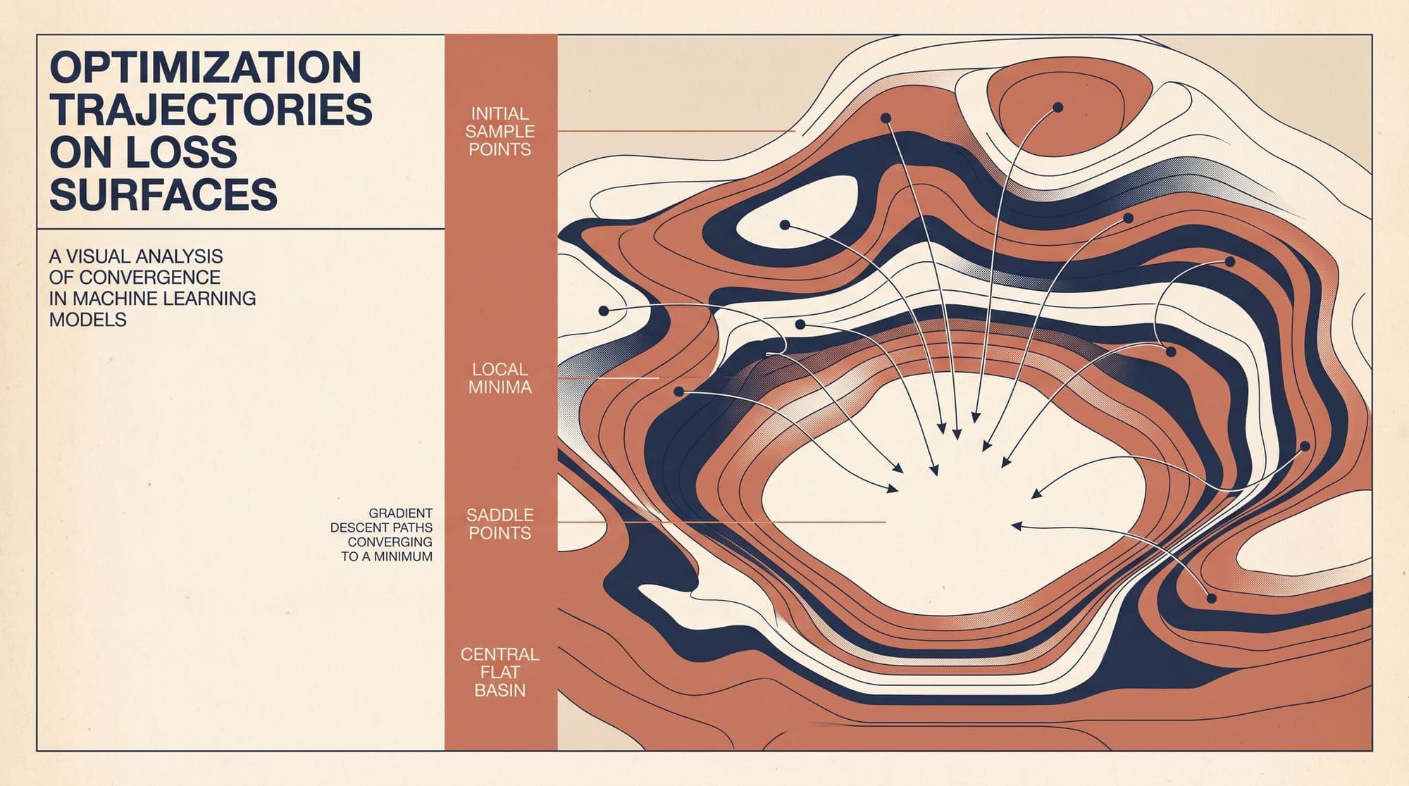
During the optimization of deep neural networks, standard Stochastic Gradient Descent (SGD) and adaptive optimizers often struggle to find solutions that generalize robustly to unseen data. While learning rate decay allows optimizers to settle into local minima on the empirical training loss surface, empirical and theoretical analyses reveal that standard gradient descent tends to halt near the boundaries of wide loss basins rather than reaching their interior.

Introduced by Izmailov et al. (2018), Stochastic Weight Averaging (SWA) resolves this disconnect by maintaining a running arithmetic average of model weights traversed during training with a cyclical or high constant learning rate. By ensembling models in parameter space rather than prediction space, SWA locates solutions situated centrally within wide, flat loss valleys. This geometric shift provides the generalization benefits of traditional ensemble methods at zero additional inference latency and negligible computational overhead.

1. The Optimization vs. Generalization Dilemma

Training deep neural networks is formulated as empirical risk minimization over a parameter space $\mathbb{R}^d$:

$$\min_{w \in \mathbb{R}^d} \mathcal{L}_{\text{train}}(w) = \frac{1}{N} \sum_{i=1}^N \ell(f(x_i; w), y_i)$$

However, the objective of deep learning is minimizing expected risk over the true data distribution $\mathcal{D}$:

$$\mathcal{L}_{\text{test}}(w) = \mathbb{E}_{(x, y) \sim \mathcal{D}} [\ell(f(x; w), y)]$$

Because the training set is a finite sample of $\mathcal{D}$, the empirical loss surface $\mathcal{L}_{\text{train}}(w)$ does not perfectly mirror $\mathcal{L}_{\text{test}}(w)$. Instead, the test loss surface is displaced by parameter shift $\Delta w$ and perturbed by curvature variations.

       Loss
        │
        │        Test Loss Basin                 Training Loss Basin
        │       ┌─────────────────┐             ┌─────────────────┐
        │      │                 │             │                 │
        │      │                 │    Shift    │   SGD Stop      │
        │      │                 │   ◄───────  │     (Boundary)  │
        │      │                 │             │         ▼       │
        │      │    SWA Center   │             │       *───┐     │
        │      │        ▼        │             │      /     \    │
        │      │        *        │             │     *       *   │
        │──────┴─────────────────┴─────────────┴─────────────────┴───────► Weights (w)

As demonstrated by Keskar et al. (2016) and Hochreiter & Schmidhuber (1997), the geometry of the selected local minimum governs generalization:

• Sharp Minima: Characterized by large eigenvalues in the loss Hessian $\nabla^2 \mathcal{L}(w)$. Small perturbations or shifts $\Delta w$ between training and test distributions lead to sharp increases in test loss.
• Flat Minima: Characterized by small Hessian eigenvalues and low local curvature. Flat regions maintain low loss even when evaluated on shifted test distributions.

When standard optimizers train with decaying learning rate schedules, the trajectory slows down and freezes at the earliest entry point along the perimeter of a low-loss basin. Because the boundary exhibits higher local curvature than the basin interior, standard SGD checkpoints remain sensitive to distribution shifts.

2. Loss Surface Geometry and Mode Connectivity

To understand why simple weight averaging succeeds, consider two geometric properties of non-convex neural network loss landscapes:

Asymmetric Loss Valleys

The loss surfaces of deep architectures contain wide, asymmetric, non-convex valleys. When an optimizer explores such a valley under a non-vanishing learning rate, the stochastic trajectory bounces along the outer periphery due to gradient noise and boundary steepness.

Because the valley is roughly convex within a local neighborhood, the arithmetic mean of points along the trajectory lies inside the basin interior:

$$w_{\text{SWA}} = \frac{1}{T} \sum_{i=1}^T w_i$$

While each individual iterate $w_i$ resides near the perimeter, their centroid $w_{\text{SWA}}$ moves toward the center of mass of the flat region, achieving substantially lower Hessian trace $\text{Tr}(H)$.

Linear and Non-Linear Mode Connectivity

Classical optimization intuition suggested that distinct local minima found by SGD were isolated by high-loss barriers. However, Garipov et al. (2018) and Draxler et al. (2018) demonstrated that local optima in overparameterized networks are connected by continuous, low-loss paths.

When checkpoints are sampled along a single optimization trajectory using cyclical or high constant learning rates, these iterates share the same basin or reside on connected valleys without intervening energy barriers. Averaging these checkpoints preserves low loss while dampening parameter-space variance.

3. The SWA Algorithmic Framework

SWA modifies the final phase of standard neural network training. Instead of decaying the learning rate to zero and selecting the final iterate, SWA transitions into an exploration and averaging phase.

Learning
  Rate (α)
    │
 α_0│───╲
    │    ╲  Standard Schedule (Warmup / Decay)
    │     ╲
α_SWA│      └───┬───┬───┬───┬───┬───┬───┬───┬───► Cyclical / Constant SWA LR
    │          │   │   │   │   │   │   │   │
    └──────────┴───┴───┴───┴───┴───┴───┴───┴───► Epochs
               ▲   ▲   ▲   ▲   ▲   ▲   ▲   ▲
            Collect checkpoints: w_1, w_2, w_3 ... -> Running Average

1. Learning Rate Schedules

SWA operates under two primary scheduling regimes once the model reaches a reasonable loss basin (typically after 75% of the total training budget):

1. Constant Learning Rate: Setting $\alpha(t) = \alpha_{\text{SWA}}$, where $\alpha_{\text{SWA}}$ is sufficiently large to maintain exploratory motion across the basin without escaping into divergent terrain.
2. Cyclical Learning Rate: Using a cyclical schedule (Smith, 2017) that periodically ramps between $\alpha_1$ and $\alpha_2$ with cycle length $c$. Checkpoints are recorded at the minimum of each cycle where the model is closest to a local optimum.

2. Checkpoint Accumulation

SWA maintains a single running average weight vector in memory, avoiding the storage overhead of saving all checkpoints:

$$w_{\text{SWA}} \leftarrow \frac{n \cdot w_{\text{SWA}} + w}{n + 1}$$

where $n$ is the number of accumulated checkpoints and $w$ is the current model weight vector. This update requires only $O(d)$ additional memory.

3. Updating Normalization Layer Statistics

A critical implementation detail concerns Batch Normalization (Ioffe & Szegedy, 2015) and other stateful normalization layers. While the weights $w_{\text{SWA}}$ represent the average of individual parameter tensors, the running mean $\mu$ and running variance $\sigma^2$ stored in Batch Normalization layers do not correspond to the linear average of individual batch statistics.

Evaluating $w_{\text{SWA}}$ directly with old running statistics causes severe performance degradation. To correct this, SWA requires a single post-training forward pass:

1. Freeze the averaged weights $w_{\text{SWA}}$.
2. Pass the training dataset through the network without computing gradients or updates.
3. Allow the Batch Normalization layers to re-estimate their running activation statistics ($\mu_{\text{SWA}}, \sigma_{\text{SWA}}^2$) directly from the activations produced by $w_{\text{SWA}}$.

import torch

def update_bn(loader, model, device):
    """Recomputes Batch Normalization statistics for an SWA model."""
    momenta = {}
    for module in model.modules():
        if isinstance(module, torch.nn.modules.batchnorm._BatchNorm):
            module.running_mean = torch.zeros_like(module.running_mean)
            module.running_var = torch.ones_like(module.running_var)
            momenta[module] = module.momentum
            module.momentum = None
            module.num_batches_tracked *= 0

    model.train()
    with torch.no_grad():
        for input, _ in loader:
            input = input.to(device)
            model(input)

    for module, momentum in momenta.items():
        module.momentum = momentum

4. Theoretical Foundations: PAC-Bayes and Curvature

The generalization advantage of SWA is formalized through PAC-Bayesian generalization theory (McAllester, 1999; Neyshabur et al., 2017).

Consider a posterior distribution $Q = \mathcal{N}(w, \sigma^2 I)$ centered at the learned weights $w$ and a prior distribution $P = \mathcal{N}(0, \sigma_0^2 I)$. The PAC-Bayes theorem bounds the expected test risk with probability at least $1 - \delta$:

$$\mathcal{L}_{\text{test}}(w) \le \mathcal{L}_{\text{train}}(w) + \sqrt{\frac{\text{KL}(Q \parallel P) + \ln(2\sqrt{N}/\delta)}{2N}}$$

Approximating the expected empirical loss under parameter perturbation via a second-order Taylor expansion gives:

$$\mathbb{E}_{v \sim \mathcal{N}(0, \sigma^2 I)} [\mathcal{L}_{\text{train}}(w + v)] \approx \mathcal{L}_{\text{train}}(w) + \frac{\sigma^2}{2} \text{Tr}\left(\nabla^2 \mathcal{L}_{\text{train}}(w)\right)$$

where $\text{Tr}(H) = \sum_{i=1}^d \lambda_i$ is the trace of the Hessian matrix.

When the Hessian trace is large (a sharp minimum), the expected perturbed loss rises rapidly, inflating the generalization bound. SWA directly reduces $\text{Tr}(H)$ by placing $w_{\text{SWA}}$ in the geometric center of the low-loss manifold, ensuring that surrounding isotropic perturbations remain within the basin of low empirical loss.

Comparative Optimization Dynamics

• Standard SGD: High Hessian trace $\text{Tr}(H)$, large max eigenvalue $\lambda_{\max}$, settles at the basin boundary, $1\times$ inference cost.
• Prediction Ensembling: Variable Hessian trace, evaluates $K$ distinct points in parameter space, multiplies inference cost by $K\times$.
• Stochastic Weight Averaging (SWA): Low Hessian trace $\text{Tr}(H)$, small max eigenvalue $\lambda_{\max}$, converges to the geometric basin centroid, $1\times$ inference cost (zero overhead).

5. Bayesian Uncertainty: SWA-Gaussian (SWAG)

Beyond point estimation, the collection of weights gathered during the SWA trajectory contains empirical information regarding the geometry of the posterior distribution $p(w \mid \mathcal{D})$.

Developed by Maddox et al. (2019), SWA-Gaussian (SWAG) uses the SGD iterates to construct a Gaussian posterior approximation without the heavy compute requirements of Markov Chain Monte Carlo (MCMC):

$$q(w) = \mathcal{N}(\mu_{\text{SWA}}, \Sigma_{\text{SWAG}})$$

Because a full $d \times d$ covariance matrix is intractable for deep networks (where $d > 10^8$), SWAG decomposes $\Sigma_{\text{SWAG}}$ into a diagonal component and a low-rank deviation matrix:

$$\Sigma_{\text{SWAG}} = \frac{1}{2} \Sigma_{\text{diag}} + \frac{1}{2(K-1)} \sum_{i=1}^K (w_i - \bar{w}_i)(w_i - \bar{w}_i)^T$$

where:

• $\Sigma_{\text{diag}} = \text{diag}(\overline{w^2} - \bar{w}^2)$ captures coordinate-wise variance.
• $K$ is the rank of the deviation matrix formed by the last $K$ recorded checkpoints.

At inference time, sampling weights $w \sim q(w)$ enables scalable Bayesian model averaging, out-of-distribution detection, and calibrated uncertainty quantification with standard network architectures.

6. Modern Evolution in Large Language Models

The core insight of SWA (that linear combinations of weights in low-loss regions yield superior generalization) has become fundamental to frontier foundation model training:

                      ┌── Model Checkpoint A ──┐
                      ├── Model Checkpoint B ──┼──► Linear / Weighted Average ──► Flatter Optimum
                      └── Model Checkpoint C ──┘     (Zero Added Latency)        (Improved Evals)

1. Model Soups

Wortsman et al. (2022) extended SWA principles to fine-tuning large vision and language models. By fine-tuning a pre-trained foundation model across diverse hyperparameter configurations (learning rates, augmentations, random seeds) and averaging their final parameter weights:

• Uniform Soup: Averages all fine-tuned checkpoints equally.
• Greedy Soup: Iteratively appends checkpoints to the average only if they improve validation accuracy.

Model soups consistently outperform single best checkpoints without requiring multiple model executions during inference.

2. Warmup-Stable-and-Merge (WSM) in LLM Pre-Training

Modern LLM pre-training frameworks increasingly replace pure cosine learning rate schedules with Warmup-Stable-Decay (WSD) schedules (Hu et al., 2024).

In architectures such as Ling-3.0 and DeepSeek-V3, the stable training phase maintains high learning rate exploration across thousands of steps. Checkpoints gathered during this stable phase or across early cooldown trajectories are combined via weight-space merging (WSM), directly leveraging SWA geometry to smooth out training loss spikes and improve zero-shot robustness across downstream evaluations.

3. Task Arithmetic and Merge Topologies

Weight averaging principles form the foundation of model merging techniques, including Task Arithmetic (Ilharco et al., 2022), TIES-Merging (Yadav et al., 2023), and DARE (Yu et al., 2023). By treating parameter vectors as directional task vectors, multi-task capabilities can be synthesized linearly without joint gradient optimization.

7. Trade-Offs and Failure Modes

While SWA is computationally lightweight, successful deployment requires adherence to specific optimization constraints:

1. The Basin Barrier Condition: SWA requires that all averaged checkpoints reside within the same connected low-loss basin. Averaging models trained from different random initializations (without permutation alignment via Git Re-Basin) traverses high-loss barriers, destroying representation capacity.
2. Exploration Learning Rate Calibration: If $\alpha_{\text{SWA}}$ is set too low, the optimizer collapses into standard SGD, sampling nearly identical points and yielding zero ensembling benefit. If $\alpha_{\text{SWA}}$ is set too high, the trajectory destabilizes and escapes the basin.
3. Normalization Desynchronization: Failing to run the post-training forward pass to re-estimate normalization layer statistics ($\mu, \sigma^2$) is the most common operational error, often reducing classification accuracy to near-random performance.
4. Memory Footprint During Training: Maintaining the running average parameter tensor requires $2\times$ the parameter memory budget during the final training phase. For trillion-parameter distributed models, SWA state tensors must be sharded across ZeRO/FSDP ranks.

Sources

• Averaging Weights Leads to Wider Optima and Better Generalization (Izmailov et al., UAI 2018)
• Loss Surfaces, Mode Connectivity, and Fast Geometric Ensembling (Garipov et al., NeurIPS 2018)
• A Simple Baseline for Bayesian Uncertainty in Deep Learning (Maddox et al., NeurIPS 2019)
• Model Soups: Averaging Weights of Multiple Fine-Tuned Models Improves Accuracy Without Increasing Inference Time (Wortsman et al., ICML 2022)
• On Large-Batch Training for Deep Learning: Generalization Gap and Sharp Minima (Keskar et al., ICLR 2017)
• Flat Minima (Hochreiter & Schmidhuber, Neural Computation 1997)
• Cyclical Learning Rates for Training Neural Networks (Smith, WACV 2017)
• Mini-Batch Gradient Descent with Compression: Warmup-Stable-Decay (Hu et al., 2024)
• Editing Models with Task Arithmetic (Ilharco et al., ICLR 2023)