Parameter-Efficient Fine-Tuning Beyond LoRA: How Adapters, Prefix Tuning, Prompt Tuning, and (IA)3 Adapt Frozen LLMs

While Low-Rank Adaptation (LoRA) and its weight-decomposed variant (DoRA) serve as the prevailing standard for adapting large language models, parameter-efficient fine-tuning (PEFT) encompasses a broader taxonomy of mathematical approaches. The core objective of PEFT is to adapt multi-billion-parameter foundation models to specialized downstream tasks while updating only a fraction (typically 0.01% to 3%) of the model parameters.

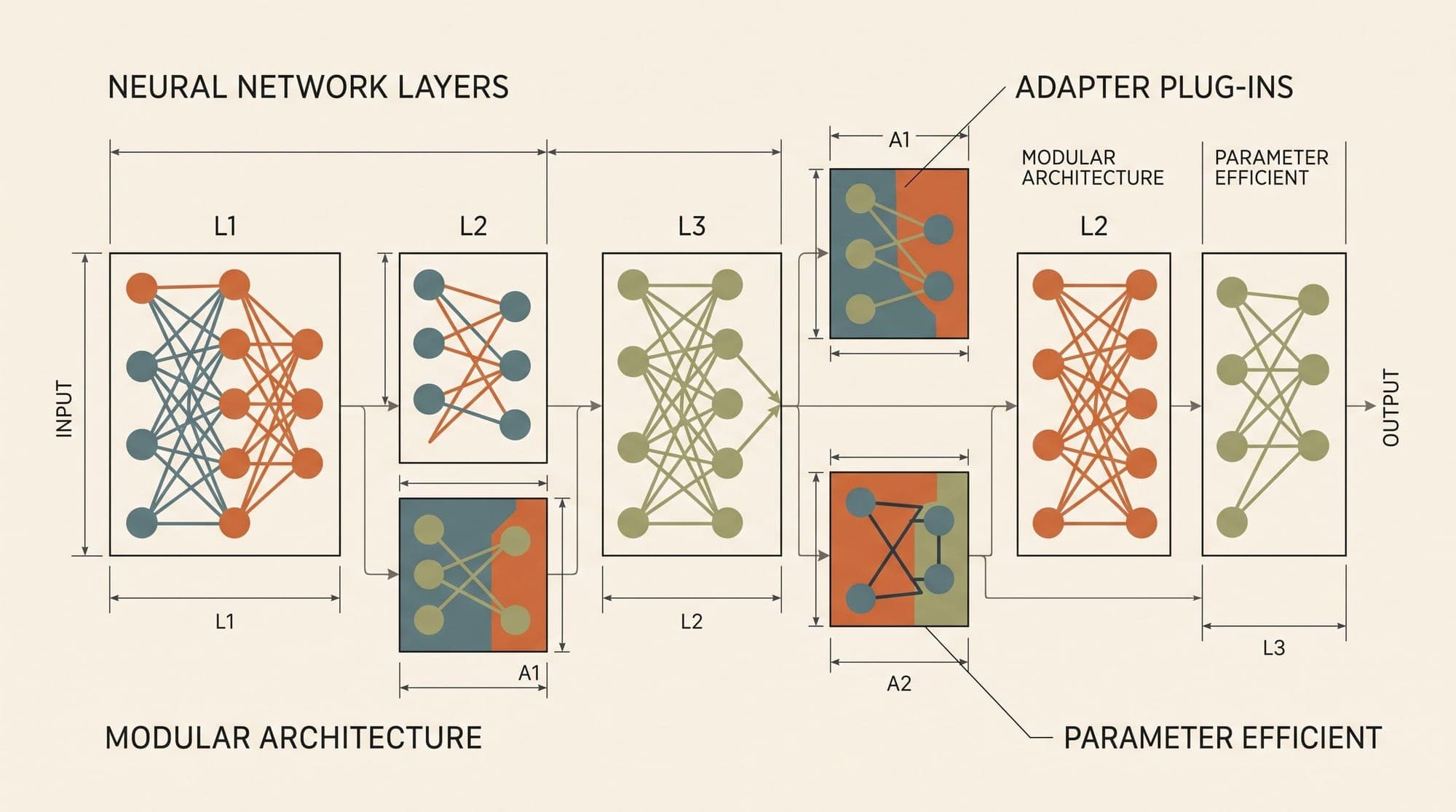
Beyond low-rank matrix decomposition, PEFT methods intervene at different points in the Transformer architecture. These techniques fall into three distinct structural paradigms: addition-based bottleneck adapters, continuous virtual activation prefixes, and multiplicative activation rescaling. Each architectural choice creates different trade-offs across trainable parameter volume, gradient stability, KV cache memory footprint, and serving latency.

1. Addition-Based PEFT: Bottleneck Adapters

Addition-based methods insert small, trainable neural sub-networks directly into the Transformer backbone while keeping all original pre-trained weights frozen.

Houlsby vs. Pfeiffer Bottleneck Adapters

The foundational adapter architecture introduced by Houlsby et al. (2019) inserts two bottleneck adapter modules into every Transformer block: one immediately after the multi-head self-attention (MHA) projection, and a second after the feedforward network (FFN) projection.

Each adapter module applies a low-dimensional bottleneck projection:

$$\text{Adapter}(h) = \sigma(h W_{\text{down}}) W_{\text{up}} + h$$

Where:

• $h \in \mathbb{R}^{d}$ is the incoming hidden state representation of hidden dimension $d$.
• $W_{\text{down}} \in \mathbb{R}^{d \times m}$ projects the representation down to a small bottleneck dimension $m$ (where $m \ll d$, often $m \in [16, 64]$).
• $\sigma(\cdot)$ is a non-linear activation function such as GeLU or ReLU.
• $W_{\text{up}} \in \mathbb{R}^{m \times d}$ projects the activated bottleneck representation back to the model dimension $d$.
• An identity residual connection bypasses the bottleneck, ensuring that if $W_{\text{down}}$ and $W_{\text{up}}$ are initialized close to zero, the module acts as an identity transform at the start of training.

Pfeiffer et al. (2020) simplified this layout in the AdapterHub framework by showing that inserting a single adapter module per Transformer block (placed exclusively after the FFN add-and-norm step) achieves downstream task performance competitive with the dual-adapter design while cutting added parameter volume by roughly 50%.

Houlsby Architecture:
Input -> LayerNorm -> MHA -> Adapter_1 -> Add/Norm -> FFN -> Adapter_2 -> Add/Norm -> Output

Pfeiffer Architecture:
Input -> LayerNorm -> MHA -> Add/Norm -> FFN -> Adapter -> Add/Norm -> Output

Parallel Adapters

In standard serial adapters, the bottleneck projection is computed sequentially after the frozen sublayer. He et al. (2021) demonstrated that bottleneck adapters can also execute in parallel alongside the frozen attention or FFN layers:

$$h_{\text{out}} = \text{FFN}(h) + s \cdot \sigma(h W_{\text{down}}) W_{\text{up}}$$

Where $s \ge 1$ is a scaling hyperparameter. Parallel adapters allow the host engine to launch the frozen layer GEMM and the adapter GEMM concurrently, mitigating some of the sequential pipeline stalls encountered in serial adapters.

Latency and Serving Trade-Offs

Because bottleneck adapters contain a non-linear activation function $\sigma(\cdot)$ between $W_{\text{down}}$ and $W_{\text{up}}$, they cannot be mathematically folded into the frozen linear weight matrices $W_0$. During inference, every token generation step must execute the adapter GEMM operations sequentially, introducing additional CUDA kernel launches and GPU memory bandwidth overhead compared to static full fine-tuning or folded LoRA checkpoints.

2. Continuous Virtual Activations: Prompt Tuning, Prefix-Tuning, and P-Tuning

Rather than inserting structural layers into the model graph, prompt and prefix methods steer the model by injecting continuous, trainable virtual token representations into the hidden states.

Prompt Tuning

Lester et al. (2021) introduced Prompt Tuning, which prepends a set of $l$ learnable continuous embedding vectors $P \in \mathbb{R}^{l \times d}$ to the sequence of token embeddings $X \in \mathbb{R}^{n \times d}$ at the input layer:

$$\tilde{X} = [P; X] \in \mathbb{R}^{(l + n) \times d}$$

The entire Transformer backbone remains frozen; only the soft prompt tensor $P$ is updated via gradient descent.

While Prompt Tuning requires minimal parameter storage (often less than 0.01% of model weights), its effectiveness is tightly tied to model scale:

• At scales exceeding 10 billion parameters, soft prompt tuning approaches the task performance of full model fine-tuning.
• At smaller scales (sub-3B parameters), prompt tuning struggles with optimization stability and expressive capacity because gradients must propagate backward through dozens of frozen layers to update only the input embeddings.

Prefix-Tuning

To resolve the depth bottleneck of prompt tuning, Li and Liang (2021) developed Prefix-Tuning. Instead of prepending virtual tokens only at the input layer, Prefix-Tuning prepends learnable prefix vectors $P_K \in \mathbb{R}^{l \times d_k}$ and $P_V \in \mathbb{R}^{l \times d_v}$ to the Key and Value representations at every attention layer:

$$K' = [P_K; K], \quad V' = [P_V; V]$$

The Multi-Head Attention computation at each layer attends over both the learnable prefix and the sequence representations:

$$\text{Attn}(Q, K', V') = \text{softmax}\left(\frac{Q [P_K; K]^T}{\sqrt{d_k}}\right) [P_V; V]$$

Prefix-Tuning Attention Flow:
Queries:  [       Q_sequence       ]
Keys:     [ P_K_virtual ; K_sequence ]
Values:   [ P_V_virtual ; V_sequence ]

Optimization Stability and Reparameterization

Optimizing the prefix parameters $P_K, P_V$ directly from random initialization leads to unstable optimization and sensitivity to learning rate selection. To stabilize training, Li and Liang reparameterized the prefix matrix through a two-layer Multi-Layer Perceptron (MLP) over a smaller latent embedding:

$$P_K, P_V = \text{MLP}_\theta(E_{\text{prefix}})$$

Once fine-tuning converges, the MLP reparameterization network is discarded; only the computed static prefix matrices $P_K, P_V$ are preserved for inference.

P-Tuning v2 (Liu et al., 2021) extended deep prefix injection across all Transformer layers for natural language understanding and generation, demonstrating that removing the MLP reparameterization is feasible across larger foundation models when using appropriate learning rate warmups and layer-wise prefix depths.

The KV Cache Penalty

Unlike weight-based fine-tuning methods, Prefix-Tuning alters the effective sequence length processed by the attention mechanism. Because $l$ prefix vectors are prepended to keys and values at every layer, every request running through a prefix-tuned model must allocate $l$ additional tokens in its KV cache across all layers. In high-concurrency production serving, this permanently consumes a portion of GPU HBM and slightly reduces the maximum batch size and effective context window available for user prompts.

3. Rescaling-Based PEFT: (IA)3 and BitFit

Rescaling methods avoid adding intermediate linear projection matrices or virtual sequence tokens. Instead, they learn low-dimensional multiplicative vectors or isolate existing sparse parameter subsets.

(IA)3: Infused Adapter by Inhibiting and Amplifying Inner Activations

Introduced by Liu et al. (2022) in the T-Few framework, $(IA)^3$ introduces learned vector scaling directly onto intermediate activation tensors:

1. Key and Value Scaling in Multi-Head Attention:

$$\text{Attn}(Q, K, V) = \text{softmax}\left(\frac{Q (l_k \odot K)^T}{\sqrt{d_k}}\right) (l_v \odot V)$$ Where $l_k \in \mathbb{R}^{d_k}$ and $l_v \in \mathbb{R}^{d_v}$ are learned scaling vectors initialized to ones, and $\odot$ denotes element-wise multiplication.

1. Intermediate Activation Scaling in Feedforward Networks:

$$\text{FFN}(x) = \left( l_{ff} \odot \sigma(x W_1) \right) W_2$$ Where $l_{ff} \in \mathbb{R}^{d_{ff}}$ scales the post-activation hidden states of the intermediate FFN projection.

(IA)3 Parameter Scaling:
Attention Keys:   K' = l_k (element-wise) * (X W_K)
Attention Values: V' = l_v (element-wise) * (X W_V)
FFN Projection:   H' = l_ff (element-wise) * sigma(X W_1)

Mathematical Weight Fusion at Zero Latency

A key property of $(IA)^3$ is that element-wise vector scaling on linear outputs is mathematically associative with the column or row dimensions of the adjacent weight matrices.

During inference deployment, the learned scaling vectors can be permanently fused into the base model weights:

$$W_K' = \text{diag}(l_k) W_K, \quad W_V' = \text{diag}(l_v) W_V, \quad W_1' = \text{diag}(l_{ff}) W_1$$

When fused, $(IA)^3$ introduces zero added inference latency, requires no additional kernel launches, and consumes zero extra KV cache memory.

Parameter Footprint

$(IA)^3$ updates only the three vectors $l_k, l_v, l_{ff}$ per Transformer layer. For an 11-billion parameter model like T0, the total trainable parameters across all layers sum to roughly 0.01% of the base model (often under 500 KB per adapter checkpoint). This compact footprint allows serving systems to store thousands of task-specific adapters in host memory and dynamically apply them on demand.

BitFit: Bias-Only Fine-Tuning

Zaken et al. (2021) introduced BitFit, an extreme baseline for parameter-efficient adaptation where all weight matrices $W$ remain frozen, and only the bias vectors $b$ across attention and FFN layers are modified:

$$h_{\text{out}} = h W_0 + (b_0 + \Delta b)$$

BitFit isolates roughly 0.05% to 0.1% of the model parameters. While it underperforms on complex multi-task benchmarks compared to $(IA)^3$ or LoRA, it demonstrates that adjusting the thresholding offsets of frozen representations accounts for a significant portion of downstream task adaptation.

4. Unified Mathematical Framework for PEFT

He et al. (2021) unified adapters, prefix tuning, and LoRA into a single functional formulation. Any parameter-efficient modification to a sublayer output $h = f(x)$ can be represented as adding a specialized delta $\Delta h$:

$$\tilde{h} = h + \Delta h$$

| PEFT Method | Mathematical Delta $\Delta h$ | Insertion Point | Fusable at Inference? | | :--- | :--- | :--- | :--- | | Houlsby / Pfeiffer Adapters | $\sigma(h W_{\text{down}}) W_{\text{up}}$ | Post-Attention / Post-FFN | No (Non-linear activation) | | Parallel Adapters | $\sigma(x W_{\text{down}}) W_{\text{up}}$ | Parallel to Sublayer | No (Non-linear activation) | | Prefix-Tuning | $\sum_i w_i (P_{V,i} - h W_V)$ | Multi-Head Attention ($K, V$) | No (Modifies KV Sequence) | | Prompt Tuning | Input embedding shift via attention | Input Layer Only | No (Prepends tokens) | | LoRA | $\frac{\alpha}{r} (x A) B$ | Linear Projections ($Q, K, V, O, W_{ff}$) | Yes ($W' = W_0 + \frac{\alpha}{r} A B$) | | $(IA)^3$ | $(l \odot \text{Act}(x)) - \text{Act}(x)$ | Keys, Values, FFN Intermediates | Yes ($W' = \text{diag}(l) W$) | | BitFit | $\Delta b$ | Bias Vectors | Yes ($b' = b_0 + \Delta b$) |

This structural unification illustrates that:

1. LoRA and $(IA)^3$ modify the linear transformation directly, enabling exact algebraic weight fusion at inference time with zero latency overhead.
2. Bottleneck Adapters introduce non-linearities, providing flexible sub-layer capacity at the cost of execution serialization and kernel overhead.
3. Prefix and Prompt Tuning modulate attention distributions through sequence-level context steering, trading KV cache capacity for parameter efficiency.

5. Architectural Comparison and Selection Criteria

Choosing between PEFT architectures depends on the operational constraints of the deployment environment:

+------------------+-------------------+--------------------+---------------------+
| Method           | Trainable Params  | KV Cache Overhead  | Inference Latency   |
+------------------+-------------------+--------------------+---------------------+
| Full Fine-Tuning | 100%              | None               | Baseline (1.0x)     |
| Houlsby Adapter  | 0.5% - 3.0%       | None               | +5% to +15%         |
| Pfeiffer Adapter | 0.2% - 1.5%       | None               | +3% to +8%          |
| Prefix-Tuning    | 0.1% - 1.0%       | +l tokens per layer| Minor (KV lookup)   |
| Prompt Tuning    | < 0.05%           | +l tokens (input)  | Minor (Prefix len)  |
| LoRA             | 0.05% - 0.5%      | None               | Zero (When fused)   |
| (IA)^3           | < 0.01%           | None               | Zero (When fused)   |
| BitFit           | 0.05% - 0.1%      | None               | Zero (When fused)   |
+------------------+-------------------+--------------------+---------------------+

Engineering Guidelines

1. High-Throughput Shared Endpoints: If hundreds of specialized tasks must run through a single inference engine without latency penalties or memory bloat, $(IA)^3$ and LoRA are optimal because their weights can be merged on-the-fly or handled via efficient multi-LoRA kernels (like S-LoRA or Punica).
2. Context-Constrained Inference: When servicing long document retrieval or large prompt windows, avoid Prefix-Tuning, as prefix tokens consume fixed slots across all KV cache layers, directly degrading maximum sequence length capacity.
3. Cross-Task Composition: If combining multiple task adapters simultaneously (e.g. AdapterFusion), Bottleneck Adapters provide modular representations that can be dynamically weighted via learned routing gates.

Sources

• Houlsby, N., et al. (2019). Parameter-Efficient Transfer Learning for NLP. arXiv:1902.00751.
• Pfeiffer, J., et al. (2020). AdapterHub: A Framework for Adapting Transformers. arXiv:2005.00349.
• Li, X. L., & Liang, P. (2021). Prefix-Tuning: Optimizing Continuous Prompts for Generation. arXiv:2101.00190.
• Lester, B., et al. (2021). The Power of Scale for Parameter-Efficient Prompt Tuning. arXiv:2104.08691.
• Liu, X., et al. (2021). P-Tuning v2: Prompt Tuning Can Be Comparable to Fine-tuning Universally Across Scales and Tasks. arXiv:2110.07602.
• Liu, H., et al. (2022). Few-Shot Parameter-Efficient Fine-Tuning is Better and Cheaper than In-Context Learning. arXiv:2205.05638.
• He, J., et al. (2021). Towards a Unified View of Parameter-Efficient Transfer Learning. arXiv:2110.04366.
• Zaken, E. B., et al. (2021). BitFit: Simple Parameter-efficient Fine-tuning for Transformer-based Masked Language-models. arXiv:2106.10199.