Odds Ratio Preference Optimization (ORPO): Mathematical Foundations, Monolithic SFT-Alignment, and Reference-Free Odds Penalties

Post-training large language models typically relies on a decoupled, two-stage pipeline: Supervised Fine-Tuning (SFT) on curated instruction-response pairs, followed by Preference Alignment using algorithms such as Reinforcement Learning from Human Feedback (PPO) or Direct Preference Optimization (DPO). While effective, this multi-stage paradigm introduces substantial operational and computational friction.

First, DPO and PPO require maintaining auxiliary reference models in GPU memory to prevent policy collapse via Kullback-Leibler (KL) divergence constraints. For large models, keeping a frozen copy of the reference model doubles the required parameter memory per device. Second, the SFT warm-up stage creates an unintended side effect: cross-entropy minimization on preferred answers inadvertently raises the log-likelihood of disfavored, low-quality responses within the same domain.

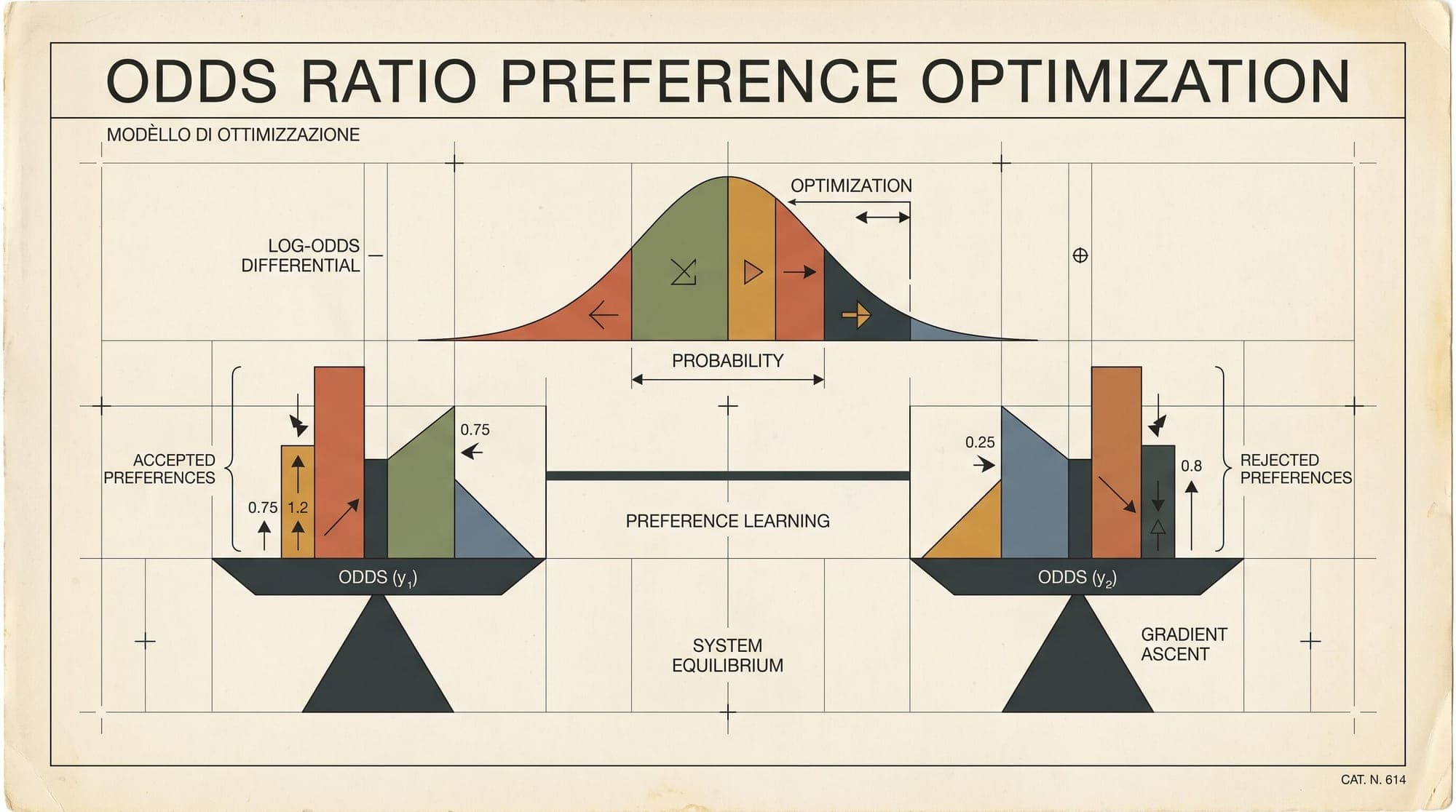
Odds Ratio Preference Optimization (ORPO), introduced by Jiwoo Hong, Noah Lee, and James Thorne at EMNLP 2024, resolves these bottlenecks by unifying supervised instruction adaptation and preference alignment into a single, reference-free monolithic objective. By appending an odds ratio penalty directly to the standard cross-entropy loss, ORPO steers model generation away from rejected styles while adapting to target task distributions in one training pass.

ORPO Monolithic Architecture and Objective Flow

The SFT Amplification Problem in Preference Tuning

The standard post-training pipeline begins by fine-tuning a base pre-trained model $\pi_\theta$ on preferred demonstrations $y_w$ given prompts $x$ using standard causal cross-entropy loss:

$\mathcal{L}_{\text{SFT}}(\theta) = -\frac{1}{|y_w|} \sum_{t=1}^{|y_w|} \log P_\theta(y_{w,t} \mid x, y_{w,<t})$

Minimizing $\mathcal{L}_{\text{SFT}}$ updates model parameters along the gradient of positive demonstrations. In high-dimensional token space, language models learn generalized representations of grammar, syntax, domain vocabulary, and formatting patterns.

However, empirical measurements demonstrate that standard SFT exerts an unconstrained upward pressure on the entire output distribution of the target domain. Because chosen responses $y_w$ and rejected responses $y_l$ frequently share vocabulary, topic entities, and sentence structure, minimizing cross-entropy on $y_w$ unintentionally increases the log-probability of rejected completions $P_\theta(y_l \mid x)$ as well.

When an unaligned SFT model is evaluated, it frequently assigns high probability to degenerate patterns, repetitive loops, or hallucinated continuations that share lexical overlap with valid training targets. Conventional alignment frameworks correct this by adding a secondary phase where a reward model or reference model regularizes the policy. ORPO demonstrates that this secondary stage is unnecessary if a contrastive odds penalty is applied during SFT itself.

Mathematical Formulation of Odds and Odds Ratios

To construct a reference-free objective, ORPO formulates sequence preference using the statistical concept of odds rather than raw token probabilities.

Sequence Probability Definition

Let $x$ represent the input prompt and $y = (y_1, y_2, \dots, y_m)$ represent an output sequence of length $m = |y|$ . The length-normalized sequence probability under model parameters $\theta$ is defined as the geometric mean of the autoregressive token conditionals:

$P_\theta(y \mid x) = \left( \prod_{t=1}^m P_\theta(y_t \mid x, y_{<t}) \right)^{\frac{1}{m}}$

In log-space, this corresponds to the average token log-likelihood:

$\log P_\theta(y \mid x) = \frac{1}{m} \sum_{t=1}^m \log P_\theta(y_t \mid x, y_{<t})$

Length normalization is critical: without dividing by sequence length $m$ , longer responses would suffer an artificial probability penalty due to repeated multiplication of numbers bounded in $[0, 1]$ , biasing the optimization toward shorter strings.

The Odds Formulation

In probability theory, the odds of an event occurring is the ratio of the probability of the event to the probability of its complement:

$\text{odds}_\theta(y \mid x) = \frac{P_\theta(y \mid x)}{1 - P_\theta(y \mid x)}$

The odds formulation provides distinct mathematical properties compared to raw probability:

When $P_\theta(y \mid x) \to 0$ , $\text{odds}_\theta(y \mid x) \approx P_\theta(y \mid x)$ .
When $P_\theta(y \mid x) \to 1$ , $\text{odds}_\theta(y \mid x) \to \infty$ .

Because the denominator $(1 - P_\theta(y \mid x))$ approaches zero as confidence grows, small gains in probability near 1 produce massive non-linear increases in odds, strongly rewarding confident preferred generations.

The Odds Ratio

Given a prompt $x$ , a winning (chosen) completion $y_w$ , and a losing (rejected) completion $y_l$ , the Odds Ratio $OR_\theta(y_w, y_l)$ quantifies how much more likely the model is to generate $y_w$ relative to $y_l$ :

$OR_\theta(y_w, y_l) = \frac{\text{odds}_\theta(y_w \mid x)}{\text{odds}_\theta(y_l \mid x)} = \frac{\frac{P_\theta(y_w \mid x)}{1 - P_\theta(y_w \mid x)}}{\frac{P_\theta(y_l \mid x)}{1 - P_\theta(y_l \mid x)}}$

Taking the logarithm yields the log odds ratio:

$\log OR_\theta(y_w, y_l) = \log \left( \frac{P_\theta(y_w \mid x)}{1 - P_\theta(y_w \mid x)} \right) - \log \left( \frac{P_\theta(y_l \mid x)}{1 - P_\theta(y_l \mid x)} \right)$

If the model assigns identical odds to both completions, $\log OR_\theta = 0$ . When the model assigns higher odds to the preferred output, $\log OR_\theta > 0$ .

The Monolithic ORPO Loss Function

ORPO optimizes a single combined objective that joins task adaptation cross-entropy with the log odds ratio penalty:

$\mathcal{L}_{\text{ORPO}}(\theta) = \mathbb{E}_{(x, y_w, y_l)} \left[ \mathcal{L}_{\text{SFT}}(\theta; x, y_w) + \lambda \cdot \mathcal{L}_{\text{OR}}(\theta; x, y_w, y_l) \right]$

where $\lambda$ is a balancing coefficient (typically selected between $0.05$ and $0.2$ ).

The odds ratio loss component $\mathcal{L}_{\text{OR}}$ is formulated as a binary cross-entropy objective wrapped in a sigmoid function:

$\mathcal{L}_{\text{OR}}(\theta; x, y_w, y_l) = -\log \sigma \left( \log OR_\theta(y_w, y_l) \right) = \log \left( 1 + e^{-\log OR_\theta(y_w, y_l)} \right)$

where $\sigma(z) = \frac{1}{1 + e^{-z}}$ is the standard logistic function.

Why ORPO Does Not Need a Reference Model

In Direct Preference Optimization (DPO), the loss is parameterized around an implicit reward function defined relative to a reference policy $\pi_{\text{ref}}$ :

$r(x, y) = \beta \log \frac{\pi_\theta(y \mid x)}{\pi_{\text{ref}}(y \mid x)}$

Without $\pi_{\text{ref}}$ , DPO's objective would degenerate: the model could satisfy the preference margin simply by driving $\log \pi_\theta(y_l \mid x) \to -\infty$ or collapsing probability mass onto arbitrary sub-tokens, destroying base generative capabilities. The reference model acts as an anchor that prevents the policy from drifting away from valid linguistic distributions.

In ORPO, the role of the anchor is fulfilled directly by the $\mathcal{L}_{\text{SFT}}$ term on $y_w$ . The cross-entropy loss continuously maximizes the likelihood of fluent, accurate, in-distribution tokens, preserving syntax and task competency. Simultaneously, $\mathcal{L}_{\text{OR}}$ acts as a regularized discriminator, penalizing the relative odds of $y_l$ without requiring a frozen second model in memory.

Gradient Dynamics and Optimization Mechanics

To examine how ORPO guides parameter updates during backpropagation, we compute the analytical gradient of the odds ratio loss component.

Gradient Derivation

The gradient of $\mathcal{L}_{\text{OR}}$ with respect to model parameters $\theta$ is:

$\nabla_\theta \mathcal{L}_{\text{OR}} = -\left(1 - \sigma(\log OR_\theta)\right) \nabla_\theta \log OR_\theta = -\sigma(-\log OR_\theta) \nabla_\theta \log OR_\theta$

We expand $\nabla_\theta \log OR_\theta$ using the derivative of the logit transformation:

$\frac{d}{dP} \log \left( \frac{P}{1 - P} \right) = \frac{d}{dP} \left( \log P - \log(1 - P) \right) = \frac{1}{P} + \frac{1}{1 - P} = \frac{1}{P(1 - P)}$

Applying the chain rule to $\nabla_\theta \log \left(\frac{P_\theta(y \mid x)}{1 - P_\theta(y \mid x)}\right)$:

$\nabla_\theta \log \left(\frac{P_\theta(y \mid x)}{1 - P_\theta(y \mid x)}\right) = \frac{1}{P_\theta(y \mid x)(1 - P_\theta(y \mid x))} \nabla_\theta P_\theta(y \mid x) = \frac{1}{1 - P_\theta(y \mid x)} \nabla_\theta \log P_\theta(y \mid x)$

Substituting this identity into the gradient of the log odds ratio yields:

$\nabla_\theta \log OR_\theta = \frac{1}{1 - P_\theta(y_w \mid x)} \nabla_\theta \log P_\theta(y_w \mid x) - \frac{1}{1 - P_\theta(y_l \mid x)} \nabla_\theta \log P_\theta(y_l \mid x)$

Combining these expressions gives the full gradient for $\mathcal{L}_{\text{ORPO}}$ :

$\nabla_\theta \mathcal{L}_{\text{ORPO}} = \nabla_\theta \mathcal{L}_{\text{SFT}} + \lambda \cdot \sigma(-\log OR_\theta) \left[ \frac{1}{1 - P_\theta(y_l \mid x)} \nabla_\theta \log P_\theta(y_l \mid x) - \frac{1}{1 - P_\theta(y_w \mid x)} \nabla_\theta \log P_\theta(y_w \mid x) \right]$

Dynamics of the Weighting Factors

The gradient formulation reveals two distinct adaptive mechanisms:

Adaptive Discrepancy Weighting ( $\sigma(-\log OR_\theta)$ ): When the model already assigns far higher odds to $y_w$ than $y_l$ ( $\log OR_\theta \gg 0$ ), $\sigma(-\log OR_\theta) \to 0$ . The odds ratio gradient diminishes to zero, preventing over-optimization on pairs where preference is already resolved and allowing pure $\mathcal{L}_{\text{SFT}}$ to govern fine-tuning. Conversely, when the model incorrectly favors the rejected output ( $\log OR_\theta < 0$ ), $\sigma(-\log OR_\theta) \to 1$ , applying maximal corrective force.
Probability-Dependent Amplification ( $\frac{1}{1 - P_\theta(y \mid x)}$ ): The scaling coefficient $\frac{1}{1 - P_\theta(y_l \mid x)}$ increases monotonically as the model assigns higher probability to the rejected response $y_l$ . If the model assigns significant probability mass to an undesired completion ( $P_\theta(y_l \mid x) \to 1$ ), the gradient multiplier surges, forcefully pushing parameters away from generating $y_l$ .

Architectural Comparison Across Alignment Frameworks

Comparing ORPO to existing post-training paradigms highlights distinct architectural trade-offs:

PPO (Schulman et al., 2017): Requires an actor policy, critic value network, frozen reference model, and separate reward model. Operates across 4 to 6 forward passes per batch with an explicit KL penalty anchor. Requires a mandatory preceding SFT warm-up stage and exhibits the highest VRAM footprint.
DPO (Rafailov et al., 2023): Eliminates explicit reward and value networks but requires maintaining a frozen reference model $\pi_{\text{ref}}$ . Operates on pairwise data $(x, y_w, y_l)$ across 4 forward passes per batch. Requires a preceding SFT warm-up stage and uses implicit KL regularization relative to $\pi_{\text{ref}}$ .
KTO (Ethayarajh et al., 2024): Eliminates the requirement for pairwise preferences by operating on unpaired binary signals $(x, y, \pm 1)$ , but still requires a frozen reference model for implicit KL anchoring and a preceding SFT stage.
SimPO (Meng et al., 2024): Eliminates the reference model by formulating an implicit reward directly normalized by sequence length and enforcing a target margin $\gamma$ . However, SimPO still presupposes an already fine-tuned SFT base model to prevent degenerate outputs.
ORPO (Hong et al., 2024): Completely reference-free and monolithic. Combines domain adaptation and preference discrimination into a single pass directly from base pre-trained weights. Requires only 2 forward passes per batch and maintains the lowest VRAM footprint.

Systems and Memory Economics in Production Training

Eliminating the reference model and unifying training into a single phase delivers immediate systems advantages for distributed cluster training:

VRAM Footprint Reduction

In standard DPO implementations using Fully Sharded Data Parallel (FSDP) or DeepSpeed ZeRO-3, the reference model $\pi_{\text{ref}}$ must remain memory-resident throughout training. While $\pi_{\text{ref}}$ requires no optimizer states or gradients, its model weights must still be sharded and broadcast during forward passes. For a 70-billion parameter model in FP16 or BF16:

Policy Model Weights: ~140 GB
Reference Model Weights: ~140 GB
Optimizer States (AdamW): ~560 GB
Total base parameter footprint: ~840 GB

Under ORPO, the elimination of $\pi_{\text{ref}}$ removes 140 GB of constant memory pressure across the cluster. This free headroom allows practitioners to increase micro-batch sizes, expand context window lengths to 8K/32K tokens, or reduce total GPU device counts.

Computational Throughput

In DPO, each training iteration requires computing logits for four forward sequences per prompt-pair: $\pi_\theta(y_w \mid x)$ , $\pi_\theta(y_l \mid x)$ , $\pi_{\text{ref}}(y_w \mid x)$ , and $\pi_{\text{ref}}(y_l \mid x)$ .

In ORPO, only two forward passes are executed: $\pi_\theta(y_w \mid x)$ and $\pi_\theta(y_l \mid x)$ . The cross-entropy loss $\mathcal{L}_{\text{SFT}}$ is computed directly from the logits of $\pi_\theta(y_w \mid x)$ , reusing the exact forward graph activations. Consequently, ORPO achieves approximately a 40% to 50% speedup in step latency compared to standard DPO.

Empirical Performance and Hyperparameter Selection

In empirical benchmarks published by Hong et al. on models ranging from Phi-2 (2.7B) to Llama-2-7B and Mistral-7B:

AlpacaEval 2.0: Mistral-7B trained with ORPO on the UltraFeedback dataset achieved a length-controlled win rate of 12.2%, outperforming both standard SFT (4.7%) and multi-stage SFT + DPO baselines (9.3%).
Instruction Following (IFEval): ORPO achieved higher prompt-level strict accuracy compared to multi-stage pipelines, avoiding the degradation in length compliance frequently observed during extended DPO runs.

Implementation Guidelines

When deploying ORPO in production post-training frameworks (such as Hugging Face TRL or Axolotl):

Weighting Factor ( $\lambda$ ): Optimal performance across standard benchmarks occurs with $\lambda \in [0.05, 0.20]$ . Setting $\lambda$ too high ( $> 0.5$ ) can suppress fluency and cause underfitting on task grammar, while setting $\lambda < 0.01$ reverts behavior to standard unaligned SFT.
Sequence Masking: Cross-entropy $\mathcal{L}_{\text{SFT}}$ must only be calculated over the response tokens $y_w$ , masking out prompt tokens $x$ with label -100. For the odds ratio calculation $\mathcal{L}_{\text{OR}}$ , token log-probabilities are averaged strictly over response lengths $|y_w|$ and $|y_l|$ .
Learning Rate Schedules: Because ORPO operates as the primary fine-tuning stage from base weights, learning rates typically follow standard SFT schedules (e.g., $5 \times 10^{-6}$ to $2 \times 10^{-5}$ with cosine decay), rather than the substantially lower learning rates ( $5 \times 10^{-7}$ ) required in secondary DPO stages.