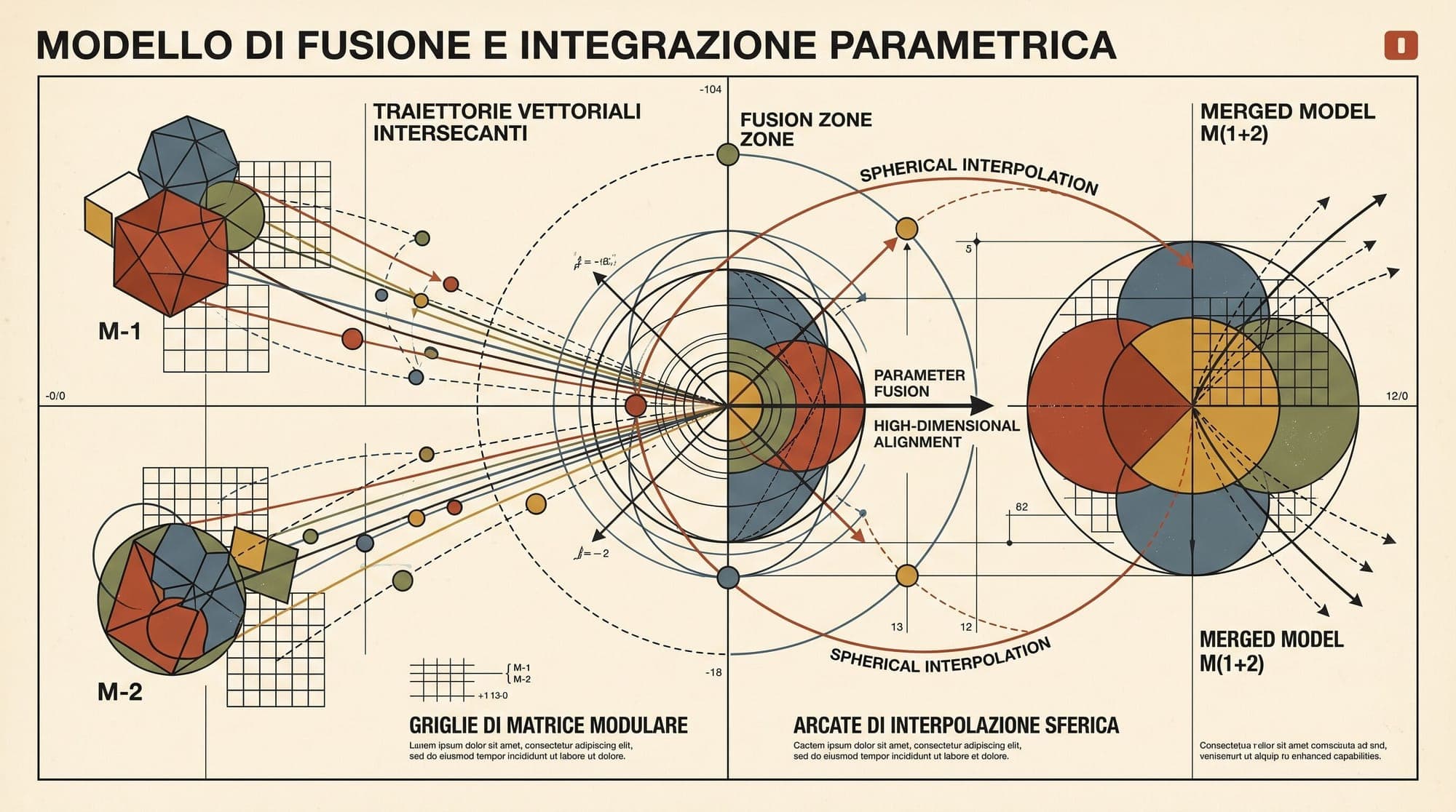
Model Merging and Task Arithmetic: Mathematical Foundations, Task Vectors, TIES-Merging, DARE, and Spherical Linear Interpolation (SLERP)

Model merging enables the combination of multiple specialized large language models into a unified checkpoint without retraining, backpropagation, or access to the original training datasets. Rather than running costly multi-task supervised fine-tuning across disparate domains, practitioners can directly manipulate parameter tensors in weight space to fuse capabilities such as mathematical reasoning, instruction following, coding, and multilingual fluency.

This explainer details the theoretical foundations and algorithms governing parameter-space fusion, from linear task vectors and spherical geometry to interference-resolving pruning techniques like TIES-Merging and DARE.

1. Parameter Geometry and Linear Mode Connectivity

Model merging relies on the empirical observation that fine-tuned neural networks derived from a shared pre-trained initialization reside within the same low-loss basin.

When models share an identical base initialization $\theta_0 \in \mathbb{R}^d$, their optimization trajectories during Supervised Fine-Tuning (SFT) remain closely aligned in the loss landscape. This phenomenon is formalized by the Linear Mode Connectivity (LMC) hypothesis (Frankle et al., 2020; Entezari et al., 2022; Ainsworth et al., 2022).

For two fine-tuned checkpoints $\theta_A$ and $\theta_B$ initialized from $\theta_0$, the linear interpolation path:

$$\theta(\alpha) = (1 - \alpha)\theta_A + \alpha \theta_B, \quad \alpha \in [0, 1]$$

often encounters virtually zero barrier in the loss surface $\mathcal{L}(\theta(\alpha))$, provided the fine-tuning step count is moderate and learning rates avoid chaotic divergence.

                       Loss Landscape Basin
                               
                      Loss L(θ)
                         ▲
                         │       Barrier for distinct inits
                         │        _ . - - - . _
                         │      /               \
                         │     /                 \
                         │    /                   \
                         │   /  Low-loss valley   \
                         │  /  (Linear Mode Conn)  \
                         │ /                       \
                         │/                         \
                         └───────●───────────●───────► Parameter Space θ
                                 θ_A         θ_B

Unlike joint multi-task training (which suffers from gradient interference, catastrophic forgetting, and immense compute overhead), weight merging operates strictly post-hoc on static parameter tensors.

2. Linear Task Arithmetic and Task Vectors

The foundational abstraction for linear parameter manipulation is the task vector, introduced by Ilharco et al. (2023).

2.1 Mathematical Formulation

Given a base model $\theta_0 \in \mathbb{R}^d$ and a model fine-tuned on task $t$, denoted $\theta_t \in \mathbb{R}^d$, the task vector $\tau_t$ is defined as the coordinate-wise delta:

$$\tau_t = \theta_t - \theta_0$$

Because $\tau_t$ represents the directional displacement in parameter space required to execute task $t$, algebraic operations on $\tau_t$ produce corresponding shifts in model capabilities:

1. Multi-Task Merging (Addition):

$$\theta_{\text{merged}} = \theta_0 + \sum_{k=1}^K \lambda_k \tau_k$$ where $\lambda_k > 0$ is a task-specific scaling hyperparameter.

1. Targeted Capability Removal (Subtraction / Unlearning):

$$\theta_{\text{unlearned}} = \theta_0 - \lambda \tau_{\text{toxic}}$$ Subtracting a task vector trained on undesirable behavior (such as toxic generations, copyrighted data, or vulnerable code) dampens those representations without full retraining.

1. Analogical Task Transfer:

$$\theta_{\text{target}} = \theta_0 + (\tau_{\text{French}} - \tau_{\text{English}})$$

2.2 Limitations of Naive Linear Addition

While elegant, naive addition of task vectors breaks down as the number of tasks $K$ grows or when fine-tuning steps push weights far from $\theta_0$. Two structural issues arise:

• Magnitude Domination: Layers with high learning-rate displacement dominate the linear sum, drowning out subtle fine-grained capabilities.
• Destructive Sign Interference: Parameter coordinates where one task vector is positive ($\tau_A^{(j)} > 0$) and another is negative ($\tau_B^{(j)} < 0$) cancel each other out, degrading performance on both source tasks.

3. Spherical Linear Interpolation (SLERP)

When merging exactly two models ($K=2$), standard Linear Interpolation (LERP) suffers from high-dimensional geometric distortion.

3.1 Geometric Shrinkage in Euclidean Interpolation

In Euclidean space, linearly interpolating between two high-dimensional vectors $\theta_A$ and $\theta_B$ of equal norm $\|\theta_A\| = \|\theta_B\| = r$ yields a midpoint whose norm is strictly smaller:

$$\|\theta(0.5)\| = \left\|\frac{\theta_A + \theta_B}{2}\right\| = r \cos\left(\frac{\Omega}{2}\right) < r$$

where $\Omega$ is the angle between $\theta_A$ and $\theta_B$. In multi-billion parameter networks, this reduction in parameter magnitude dampens activation variance across transformer layers, leading to degraded perplexity.

       LERP (Euclidean Chord) vs SLERP (Spherical Arc)
       
                     SLERP Path (Constant Norm)
                           .-'""'-.
                        .-'        '-.
                     .-'              '-.
                 θ_A ●───────────────────● θ_B
                      \   LERP Chord    /
                       \ (Norm Drops)  /
                        \             /
                         \     Ω     /
                          \    │    /
                           \   │   /
                            \  │  /
                             \ │ /
                              \│/
                               ● Origin (0,0)

3.2 SLERP Derivation

Spherical Linear Interpolation (Shoemake, 1985; adapted to LLMs by Goddard et al., 2024) traverses the great circle arc connecting the two normalized parameter vectors on a hypersphere.

Let $v_A = \frac{\theta_A}{\|\theta_A\|}$ and $v_B = \frac{\theta_B}{\|\theta_B\|}$. The angle $\Omega$ between them is:

$$\Omega = \arccos\left(\frac{v_A \cdot v_B}{\|v_A\| \|v_B\|}\right) = \arccos(v_A^T v_B)$$

The interpolated unit vector $v(t)$ for interpolation factor $t \in [0, 1]$ is:

$$\text{SLERP}(v_A, v_B; t) = \frac{\sin((1 - t)\Omega)}{\sin \Omega} v_A + \frac{\sin(t \Omega)}{\sin \Omega} v_B$$

The final parameter tensor $\theta(t)$ scales $v(t)$ by interpolating the original vector magnitudes:

$$\theta(t) = \left[ (1 - t)\|\theta_A\| + t\|\theta_B\| \right] \cdot \text{SLERP}(v_A, v_B; t)$$

By preserving angular velocity and vector norm, SLERP maintains layer activation statistics and outperforms linear averaging on pairwise model combinations.

4. TIES-Merging: Trimming, Electing Sign, and Disjoint Merging

To scale model merging to $K > 2$ models without destructive interference, Yadav et al. (NeurIPS 2023) introduced TIES-Merging (TRIM, ELECT SIGN & MERGE).

TIES identifies two primary drivers of degradation during multi-task fusion:

1. Parameter Redundancy: A vast majority of parameter changes in $\tau_k$ consist of small, low-magnitude noise accumulated during gradient descent that contribute little to downstream capability.
2. Sign Disagreements: When different task vectors push the same parameter coordinate in opposing directions ($+ \text{ vs } -$), standard averaging cancels both signals.

4.1 The Three-Stage TIES Algorithm

For a set of $K$ fine-tuned models with task vectors $\{\tau_1, \tau_2, \dots, \tau_K\}$ relative to base initialization $\theta_0$:

Step 1: Trim (Sparsification)

For each task vector $\tau_k$, retain only the top-$p\%$ elements by absolute magnitude (typically $p \in [10\%, 30\%]$). All remaining coordinates are reset to zero:

$$\hat{\tau}_k^{(j)} = \begin{cases} \tau_k^{(j)} & \text{if } |\tau_k^{(j)}| \ge \text{Quantile}_{1-p}(|\tau_k|) \\ 0 & \text{otherwise} \end{cases}$$

Step 2: Elect Sign (Directional Consensus)

For each parameter index $j \in \{1, \dots, d\}$, compute the majority directional vector $\gamma^{(j)} \in \{-1, +1\}$ across all trimmed task vectors based on total coordinate mass:

$$\gamma^{(j)} = \text{sgn}\left(\sum_{k=1}^K \hat{\tau}_k^{(j)}\right)$$

If the sum is zero, $\gamma^{(j)}$ defaults to $\text{sgn}\left(\sum_{k=1}^K \tau_k^{(j)}\right)$.

Step 3: Disjoint Merge (Selective Averaging)

For each coordinate $j$, compute the average strictly among task vectors whose sign matches the elected majority $\gamma^{(j)}$. Vectors with opposing signs are excluded for that coordinate:

$$A^{(j)} = \left\{ k \in \{1, \dots, K\} \mid \hat{\tau}_k^{(j)} \neq 0 \text{ and } \text{sgn}(\hat{\tau}_k^{(j)}) = \gamma^{(j)} \right\}$$

$$\tau_{\text{TIES}}^{(j)} = \begin{cases} \frac{1}{|A^{(j)}|} \sum_{k \in A^{(j)}} \hat{\tau}_k^{(j)} & \text{if } |A^{(j)}| > 0 \\ 0 & \text{otherwise} \end{cases}$$

The final merged model is constructed with global scaling factor $\lambda$:

$$\theta_{\text{merged}} = \theta_0 + \lambda \cdot \tau_{\text{TIES}}$$

By pruning low-magnitude updates and filtering directional conflicts, TIES eliminates destructive interference while retaining high-confidence domain updates.

5. DARE: Drop And REscale

While TIES trims by deterministic top-$k$ magnitude, Yu et al. (ICML 2024) proved in DARE (Drop And REscale) that fine-tuned delta parameters exhibit extreme structural redundancy.

5.1 The Super Mario Phenomenon

Yu et al. discovered that between 90% and 99% of delta parameters in SFT models can be set to zero at random without degrading model performance, as long as the remaining parameters are rescaled to maintain expected activation outputs.

5.2 Mathematical Formulation

Given task vector $\tau_k = \theta_k - \theta_0$ and drop rate $p \in [0.90, 0.99]$:

1. Sample a random binary mask $m_k^{(j)} \sim \text{Bernoulli}(1 - p)$ for each coordinate $j$.
2. Compute the sparsified, rescaled delta vector $\tilde{\tau}_k$:

$$\tilde{\tau}_k^{(j)} = \frac{m_k^{(j)}}{1 - p} \cdot \tau_k^{(j)}$$

Because $\mathbb{E}[m_k^{(j)}] = 1 - p$, the mathematical expectation of the rescaled vector is unbiased:

$$\mathbb{E}[\tilde{\tau}_k^{(j)}] = \frac{\mathbb{E}[m_k^{(j)}]}{1 - p} \cdot \tau_k^{(j)} = \tau_k^{(j)}$$

                   DARE Sparsification & Rescaling
                   
Original Delta:   [ +0.04 ,  -0.02 ,  +0.08 ,  -0.05 ,  +0.01 ]
Bernoulli Mask:   [   1   ,    0   ,    0   ,    1   ,    0   ]  (p = 0.6)
Dropped Delta:    [ +0.04 ,    0   ,    0   ,  -0.05 ,    0   ]
Rescaled (x 2.5): [ +0.10 ,    0   ,    0   ,  -0.125,    0   ]

5.3 DARE-TIES and DARE-Task Arithmetic

DARE is routinely paired with downstream merge algorithms:

• DARE-Task Arithmetic: Sparsify each delta with DARE, then sum: $\theta_0 + \lambda \sum_k \tilde{\tau}_k$.
• DARE-TIES: Sparsify each delta with DARE, then pass the surviving coordinates through TIES sign election and disjoint averaging.

By eliminating up to 99% of non-zero coordinates before merging, DARE drastically reduces coordinate overlap between models, lowering collision probability to near zero.

6. Advanced Merging Architectures and Evolutionary Search

Beyond weight averaging within identical layer topologies, recent advances explore cross-layer stacking and automated parameter discovery.

6.1 Model Soups

Introduced by Wortsman et al. (ICML 2022), Model Soups average the weights of multiple models fine-tuned with different hyperparameters (learning rates, random seeds, augmentations) from the same base model:

• Uniform Soup: Direct arithmetic mean $\frac{1}{K} \sum_{k=1}^K \theta_k$.
• Greedy Soup: Sequentially adds candidate checkpoints to the running average only if validation performance improves.

6.2 Passthrough / Frankenmerging (Layer Stacking)

Passthrough merging stitches layers from one or more models into non-standard depth configurations (for example, creating a 120-billion parameter model by repeating middle layers of a 70B checkpoint).

While effective at increasing capacity, frankenmerges introduce layer-to-layer hidden state distribution shifts, requiring careful interpolation across boundary layers.

6.3 Evolutionary Model Merging (Sakana AI)

Akiba et al. (2024) automated the discovery of merge configurations using evolutionary algorithms (specifically CMA-ES). Evolutionary merging operates in two spaces:

1. Parameter Space (Layer-Wise Merging): Optimizes layer-by-layer mixing coefficients $\mathbf{w}_l$ to balance task contributions across depth.
2. Data-Flow Space (Cross-Layer Routing): Optimizes inference-time activation pathways through layers of disparate models.

7. Comparative Method Matrix

| Method | Number of Models ($K$) | Sparsification Strategy | Conflict Resolution | Primary Strength | Key Limitation | | :--- | :--- | :--- | :--- | :--- | :--- | | Linear (LERP) | Arbitrary ($K \ge 2$) | None | Simple weighted average | Fast, zero hyperparameter tuning | Severe destructive sign interference | | SLERP | Pairwise ($K = 2$) | None | Hyperspherical arc interpolation | Preserves weight norm and activation variance | Restricted to pairwise merges | | Task Arithmetic | Arbitrary ($K \ge 2$) | Optional manual scaling | Linear delta addition | Supports capability subtraction/unlearning | Fragile to magnitude disparities | | TIES-Merging | Arbitrary ($K \ge 2$) | Deterministic top-$k\%$ magnitude trim | Majority sign election + disjoint mean | Eliminates gradient clashes and noise | Requires tuning trim ratio $p$ and weight $\lambda$ | | DARE-TIES | Arbitrary ($K \ge 2$) | Random Bernoulli drop ($p \in [0.9, 0.99]$) + rescaling | Majority sign election + disjoint mean | Minimal inter-model parameter collision | Non-deterministic sampling variance |

8. Implementation and Practical Engineering Recipes

Practical model merging is standardized around open-source tools such as MergeKit (Goddard et al., 2024). MergeKit executes out-of-core merging by streaming layer tensors from disk, enabling multi-model 70B merges on consumer GPUs or CPU RAM.

8.1 Example MergeKit Configuration: DARE-TIES

Below is a declarative YAML specification combining a general instruction model, a math specialist, and a coding specialist using DARE-TIES:

models:
  - model: mistralai/Mistral-7B-v0.1
    # Base model provided as reference initialization
  - model: WizardLM/WizardMath-7B-V1.1
    parameters:
      density: 0.5
      weight: 0.3
  - model: deepseek-ai/deepseek-coder-7b-instruct
    parameters:
      density: 0.5
      weight: 0.4
  - model: mistralai/Mistral-7B-Instruct-v0.2
    parameters:
      density: 0.5
      weight: 0.3

merge_method: dare_ties
base_model: mistralai/Mistral-7B-v0.1
parameters:
  int8_mask: true
dtype: bfloat16

8.2 Critical Engineering Prerequisites

1. Strict Lineage Homogeneity: All merged models must share the exact same base model architecture and tokenizer vocabulary. Merging a Llama-3-derived checkpoint with a Mistral checkpoint causes complete representational collapse due to incompatible embedding indices and attention dimensions.
2. Tokenizer Alignment: If fine-tuned models extended the special token vocabulary (e.g., adding distinct chat formatting tags), token embeddings must be reconciled or mapped prior to weight fusion.
3. Safety Alignment Drift: Merging a safety-tuned model with an uncensored domain expert frequently dilutes safety guardrails, requiring post-merge evaluation across jailbreak and toxicity benchmarks.

Sources

• Ilharco, G., et al. (2023). Editing Models with Task Arithmetic. ICLR 2023. arXiv:2212.04089
• Yadav, P., Tam, D., Choshen, L., Raffel, C., & Bansal, M. (2023). TIES-Merging: Resolving Interference When Merging Models. NeurIPS 2023. arXiv:2306.01708
• Yu, L., Yu, B., Yu, H., Huang, F., & Li, Y. (2024). Language Models are Super Mario: Absorbing Abilities from Homologous Models as a Free Lunch. ICML 2024. arXiv:2311.03099
• Goddard, C., Siriwardhana, S., Rengarajan, M., et al. (2024). Arcee's MergeKit: A Toolkit for Merging Large Language Models. arXiv:2403.13257
• Wortsman, M., et al. (2022). Model Soups: Averaging Weights of Multiple Fine-Tuned Models Improves Accuracy Without Increasing Inference Time. ICML 2022. arXiv:2203.05482
• Akiba, T., Shing, M., Tang, Y., Sun, Q., & Ha, D. (2024). Evolutionary Optimization of Model Merging Recipes. Nature Communications / arXiv:2403.13187
• Frankle, J., Dziugaite, G. K., Roy, D., & Carbin, M. (2020). Linear Mode Connectivity and the Lottery Ticket Hypothesis. ICML 2020. arXiv:2003.04887