Low-Rank Adaptation (LoRA) and QLoRA: Mathematical Foundations, Intrinsic Rank Parameterization, NF4 Quantization, and Double Quantization Mechanics

Parameter-efficient fine-tuning (PEFT) has become the standard operational methodology for adapting large language models to domain-specific tasks, downstream instruction following, and structured tool use. Full-parameter fine-tuning of frontier architectures requires updating and tracking optimizer states for tens or hundreds of billions of parameters, demanding multi-terabyte GPU clusters merely to compute backward passes.

Low-Rank Adaptation (LoRA), introduced by Hu et al. (2021), and its quantized extension QLoRA, introduced by Dettmers et al. (2023), reformulate model adaptation by freezing the base model weights and training low-rank decomposed projection matrices. This architectural paradigm reduces trainable parameter counts by over 99%, slashes optimizer memory consumption, and maintains zero inference latency overhead through weight matrix folding.

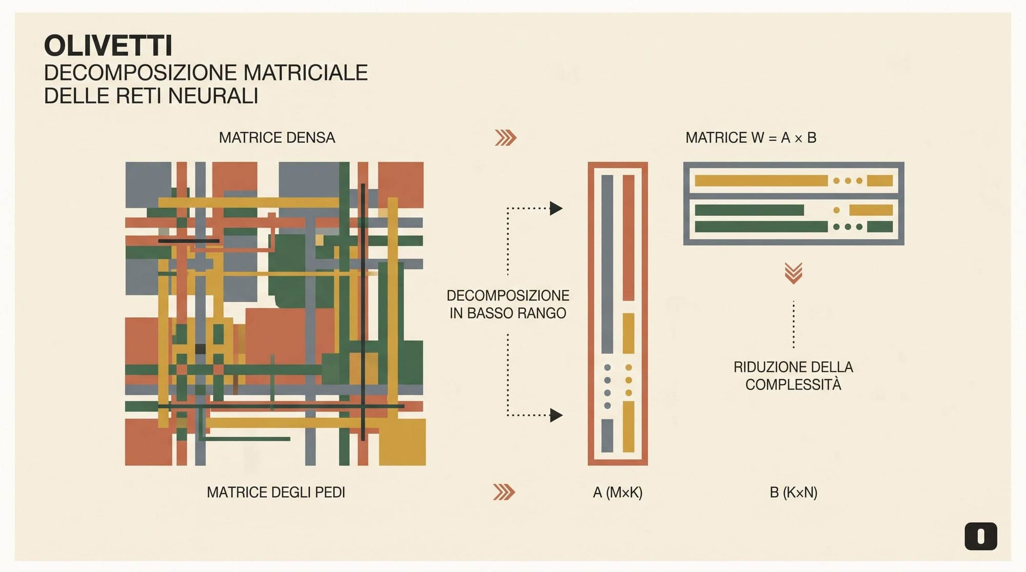
<p><img src="https://cms.llms.blog/content/images/2026/08/lora-illustration.png" alt="Low-Rank Matrix Decomposition and Quantization Architecture" /></p>

The Memory Footprint of Full-Parameter Fine-Tuning

To understand the necessity of low-rank parameterization, consider the memory allocation required during standard full-parameter fine-tuning with 16-bit mixed-precision and the standard AdamW optimizer.

For a model with $N$ parameters, the static memory footprint is divided across several distinct components:

1. Model Parameters: 16-bit floating-point weights (FP16 or BF16) require $2N$ bytes.
2. Gradients: First-order gradients computed during backpropagation require $2N$ bytes.
3. Optimizer States: AdamW maintains a master copy of weights in FP32 ($4N$ bytes), a first-moment vector (momentum, $4N$ bytes), and a second-moment vector (uncentered variance, $4N$ bytes), totaling $12N$ bytes.
4. Activations and Working Memory: Intermediate activation tensors stored for backpropagation, sequence caching, and CUDA kernel workspaces.

For a 70-billion parameter model ($N = 70 \times 10^9$), the static parameter and optimizer memory alone totals:

$$M_{\text{static}} = (2 + 2 + 12) \times 70 \times 10^9 \text{ bytes} = 1.12 \text{ TB}$$

This calculation excludes dynamic activation memory. Consequently, full fine-tuning of a 70B parameter model requires distributed sharding architectures such as Fully Sharded Data Parallel (FSDP) or DeepSpeed ZeRO-3 across at least two 8xH100 (80GB) nodes.

The Intrinsic Rank Hypothesis and Mathematical Formulation

LoRA builds on empirical findings from Aghajanyan et al. (2020), which demonstrated that overparameterized neural networks reside on a low intrinsic dimension. The manifold of parameter trajectories during downstream adaptation can be effectively approximated within a significantly lower-dimensional subspace without degrading task performance.

Matrix Factorization Formulation

Given a pre-trained linear projection weight matrix $W_0 \in \mathbb{R}^{d \times k}$, full fine-tuning optimizes an unconstrained parameter update matrix $\Delta W \in \mathbb{R}^{d \times k}$:

$$W = W_0 + \Delta W$$

LoRA parameterizes the accumulated update $\Delta W$ as the product of two low-rank matrices $B$ and $A$:

$$\Delta W = \frac{\alpha}{r} B A$$

where:

• $B \in \mathbb{R}^{d \times r}$
• $A \in \mathbb{R}^{r \times k}$
• $r \ll \min(d, k)$ is the chosen rank hyperparameter
• $\alpha \in \mathbb{R}^+$ is a constant scaling hyperparameter

During the forward pass with input representation $x \in \mathbb{R}^{b \times s \times k}$ (batch size $b$, sequence length $s$), the linear layer computes:

$$h = W_0 x + \Delta W x = W_0 x + \frac{\alpha}{r} B A x$$

Because matrix multiplication is associative, the computation of $\Delta W x$ evaluates as $(B(Ax))$. The FLOP complexity of the low-rank branch is $\mathcal{O}(b \cdot s \cdot (k \cdot r + r \cdot d))$, compared to $\mathcal{O}(b \cdot s \cdot k \cdot d)$ for a full-rank matrix multiplication. When $r = 16$ and $d = k = 4096$, the parameter count for that linear layer drops from $16,777,216$ to $131,072$, a 99.2% reduction.

Input x [d_in]
   │
   ├───> [Frozen Pre-trained Weight W_0 (d_out x d_in)] ───> h_base [d_out]
   │                                                             │
   └───> [Trainable Down-projection A (r x d_in)]                │
              │                                                  │
              ▼                                                  │
         Intermediate [r]                                        │
              │                                                  │
              ▼                                                  │
         [Trainable Up-projection B (d_out x r)]                 │
              │                                                  │
              ▼                                                  │
         Adapter Output [d_out] * (alpha / r) ───────────────────( + )
                                                                 │
                                                                 ▼
                                                            Output h [d_out]

Initialization Dynamics

To ensure that the adapter introduces zero perturbation to the pre-trained model at the start of training, the initialization of $A$ and $B$ is asymmetric:

1. Matrix $A$ is initialized using a random Gaussian distribution: $A \sim \mathcal{N}\left(0, \sigma^2\right)$ (or Kaiming uniform initialization).
2. Matrix $B$ is initialized to exact zeros: $B = 0$.

At step $t = 0$:

$$\Delta W = \frac{\alpha}{r} B A = \frac{\alpha}{r} (0) A = 0$$

Therefore, $h = W_0 x$, preserving the base model output identically until gradient updates modify $B$.

Scaling Factor Alpha and Learning Dynamics

The scaling factor $\frac{\alpha}{r}$ serves to decouple the learning rate from the choice of rank $r$. When $r$ is varied during hyperparameter sweeps, scaling $\Delta W$ by $\frac{\alpha}{r}$ stabilizes the expected magnitude of the initialization gradients and weight updates. In practice, setting $\alpha = 2r$ or $\alpha = r$ is standard; setting $\alpha$ constant ensures that changing $r$ does not require re-tuning the optimizer learning rate.

Backpropagation and Memory Mechanics

During backward propagation, the pre-trained base matrix $W_0$ remains frozen. No gradients are calculated for $W_0$, and no optimizer momentum or variance statistics are allocated for its parameters.

Given the loss function $\mathcal{L}$, the gradients with respect to $A$ and $B$ are derived via the chain rule:

$$\frac{\partial \mathcal{L}}{\partial B} = \frac{\alpha}{r} \left(\frac{\partial \mathcal{L}}{\partial h}\right)^T (A x)$$

$$\frac{\partial \mathcal{L}}{\partial A} = \frac{\alpha}{r} B^T \left(\frac{\partial \mathcal{L}}{\partial h}\right) x^T$$

The AdamW optimizer states only track the elements of $A$ and $B$. For a 70B parameter model adapted at rank $r = 16$ across all linear layers, the total trainable adapter parameters $N_{\text{adapter}}$ typically number between 100M and 250M parameters (under 0.35% of $N$). The optimizer memory drops from 1.12 TB to under 4 GB.

Target Modules and Subspace Overlap

Initial implementations of LoRA restricted adapter insertion to multi-head self-attention projection matrices: the query matrix $W_q$ and value matrix $W_v$. Subsequent empirical analyses, notably by Hu et al. (2021) and Dettmers et al. (2023), showed that targeting all linear layers yields superior adaptation capacity.

In modern Transformer architectures (such as LLaMA, Mistral, and Qwen), adapters are typically placed on:

• Self-Attention Projections: Query ($W_q$), Key ($W_k$), Value ($W_v$), and Output ($W_o$).
• Multi-Layer Perceptron (MLP) Projections: Gate ($W_{\text{gate}}$), Up ($W_{\text{up}}$), and Down ($W_{\text{down}}$).

Empirical evaluations show that adapting all seven linear modules at a low rank (such as $r = 8$ or $r = 16$) consistently outperforms adapting only $W_q$ and $W_v$ at a high rank (such as $r = 64$ or $r = 128$), while utilizing comparable parameter budgets. This occurs because domain adaptation requires distributed representations across both routing/attention mechanisms and factual/associative knowledge stored in the feed-forward blocks.

Zero-Latency Inference Folding and Multi-Tenant Serving

A critical operational advantage of LoRA over traditional bottleneck adapters (such as Houlsby or Pfeiffer architectures) is the elimination of inference latency.

Static Weight Folding

For single-tenant deployment, the low-rank delta $\Delta W$ can be merged directly into the base weights prior to inference:

$$W_{\text{merged}} = W_0 + \frac{\alpha}{r} B A$$

The resulting $W_{\text{merged}} \in \mathbb{R}^{d \times k}$ matches the dimensions of the original model layer. The model architecture at runtime is identical to the unadapted base model, with zero added parameters, zero extra kernel calls, and zero latency overhead. If task switching is required, the adapter weights can be subtracted: $W_0 = W_{\text{merged}} - \frac{\alpha}{r} B A$.

Dynamic Multi-LoRA Batching

In high-throughput multi-tenant environments where thousands of customized user adapters share a single base model, dynamic multi-LoRA inference systems (such as S-LoRA, Punica, and vLLM Multi-LoRA) maintain $W_0$ in GPU memory once. Each request in a heterogeneous batch computes $W_0 x$ via a unified batched GEMM, while the adapter paths $(B_i A_i x)$ are executed using segmented gather/scatter matrix kernels (such as Segmented GEMM / Batched-Gather-GEMM).

QLoRA: Quantized Base Weights and Memory Optimization

While LoRA eliminates optimizer memory for the base model, the static memory footprint of $W_0$ (140 GB in FP16 for a 70B model) still prevents fine-tuning on single consumer or workstation GPUs. QLoRA (Dettmers et al., 2023) resolved this bottleneck through three algorithmic innovations: NormalFloat4 (NF4) quantization, Double Quantization (DQ), and Paged Optimizers.

       ┌────────────────────────────────────────────────────────┐
       │                   QLoRA Memory Layout                  │
       └────────────────────────────────────────────────────────┘
                                   │
        ┌──────────────────────────┴──────────────────────────┐
        ▼                                                     ▼
┌───────────────────────────────┐             ┌───────────────────────────────┐
│     Base Weights: 4-bit       │             │       Adapters: 16-bit        │
│  - Storage: NF4 Quantized     │             │  - Precision: BF16 / FP16     │
│  - Double Quantization (DQ)   │             │  - Full Backward Gradients    │
│  - Frozen (No Gradients)      │             │  - AdamW Optimizer States     │
└───────────────────────────────┘             └───────────────────────────────┘
        │                                                     │
        ▼ (On-the-fly dequantization in SRAM)                 ▼
┌─────────────────────────────────────────────────────────────────────────────┐
│                       Forward Computation: BF16 GEMM                        │
│             h = dequantize(W_NF4, c1, c2) * x + (alpha / r) * B * A * x     │
└─────────────────────────────────────────────────────────────────────────────┘

1. NormalFloat4 (NF4) Data Type

Standard integer (Int4) and floating-point (FP4) quantization schemes assume uniform or arbitrary distributions over input tensors. However, pre-trained neural network weights typically follow a normal distribution centered at zero: $\mathcal{N}(0, \sigma^2)$.

NF4 is an information-theoretically optimal quantile quantization data type for normally distributed data. It constructs $2^k$ (for $k=4$, 16) discrete quantization bins such that each bin contains an equal expected number of parameter points from a standardized Gaussian distribution $\mathcal{N}(0, 1)$.

The quantile boundaries $q_i$ are computed via the standard normal cumulative distribution function (CDF) $\Phi(x)$:

$$q_i = \Phi^{-1}\left(\frac{i}{2^k}\right), \quad i \in \{0, 1, \dots, 2^k\}$$

The 16 representative values $v_i$ for NF4 are defined by the midpoints of adjacent quantiles, normalized so that the maximum absolute value is exactly $1.0$:

$$v_i = \frac{1}{2} \left[ \Phi^{-1}\left(\frac{2i - 1}{2^{k+1}}\right) + \Phi^{-1}\left(\frac{2i + 1}{2^{k+1}}\right) \right]$$

To eliminate asymmetric zero-offset errors without dedicating a bit to zero, the distribution is mapped separately for negative and positive ranges, yielding an exact zero point representation ($v_i = 0$). This ensures equal empirical coverage per bit, maximizing information entropy.

2. Double Quantization (DQ)

Block-wise quantization divides a weight tensor into blocks of size $B_1$ (typically $B_1 = 64$) and computes a 32-bit floating-point scaling constant $c_1$ per block:

$$W^{\text{quantized}} = \text{round}\left(\frac{W}{c_1}\right), \quad c_1 = \max(|W_{\text{block}}|)$$

While block size 64 controls outlier distortion, the scaling constants themselves consume substantial memory:

$$\text{Memory Overhead}_{c_1} = \frac{32 \text{ bits}}{64 \text{ weights}} = 0.5 \text{ bits per parameter}$$

Double Quantization treats the first-level scaling constants $c_1$ as inputs to a second quantization pass. The scaling factors $c_1$ are grouped into secondary blocks of size $B_2 = 256$ and quantized to 8-bit integers with a secondary FP32 scale $c_2$ and mean $\mu_2$:

$$c_1^{\text{quantized}} = \text{quantize}_{8\text{-bit}}(c_1, c_2, \mu_2)$$

The memory footprint for quantization constants drops:

$$\text{Memory Overhead}_{\text{DQ}} = \frac{8 \text{ bits}}{64} + \frac{32 \text{ bits}}{64 \times 256} = 0.125 + 0.00195 = 0.127 \text{ bits per parameter}$$

This achieves a net reduction of $0.373$ bits per parameter, saving roughly 3 GB of VRAM on a 65B/70B model with zero measurable impact on task accuracy.

3. Paged Optimizers

During training on long sequences with activation checkpointing, transient memory allocation spikes can exceed GPU VRAM capacity, triggering Out-Of-Memory (OOM) crashes. QLoRA utilizes CUDA Unified Memory to allocate optimizer state memory in paged address spaces. When allocation demands spike during the backward pass, page tables automatically evict inactive optimizer states from GPU VRAM to physical CPU RAM, fetching them back asynchronously when the optimizer step executes.

Dequantization Mechanics During Computation

Base model weights are never stored in uncompressed 16-bit format in high-bandwidth memory (HBM). Instead, base weights remain stored in 4-bit NF4. During matrix multiplication inside custom CUDA kernels:

1. A block of 4-bit NF4 weights and its quantized scaling constants are fetched into GPU Shared Memory (SRAM) and register files.
2. The scale constant is dequantized: $c_1 = c_1^{\text{quantized}} \cdot c_2 + \mu_2$.
3. The 4-bit weights are mapped via lookup table to 16-bit BF16 values: $\hat{W} = c_1 \cdot \text{LUT}_{\text{NF4}}[W_{\text{NF4}}]$.
4. Standard BF16 tensor core matrix multiplication executes with input activations $x$.
5. The low-rank branch $(B A x)$ evaluates in 16-bit precision and is added element-wise to the base branch output.

Because the dequantization occurs entirely within high-speed register files and SRAM, memory bus bandwidth usage remains bounded by the 4-bit footprint.

Structural Variants: DoRA and AdaLoRA

Several architectural extensions have built upon the foundational LoRA formulation:

Weight-Decomposed Low-Rank Adaptation (DoRA)

Introduced by Liu et al. (2024), DoRA decomposes the weight matrix into its directional component and magnitude scalar:

$$W = m \frac{W_0 + \Delta W}{\|W_0 + \Delta W\|_F} = m \frac{W_0 + \frac{\alpha}{r} B A}{\|W_0 + \frac{\alpha}{r} B A\|_F}$$

where $m \in \mathbb{R}^{1 \times k}$ is a trainable magnitude vector initialized to $m = \|W_0\|_F$, and the direction is updated via low-rank matrices $B$ and $A$. By separating directional updates from magnitude scaling, DoRA mimics the gradient dynamics of full-parameter fine-tuning more closely, achieving higher performance on reasoning benchmarks.

Adaptive Low-Rank Adaptation (AdaLoRA)

Introduced by Zhang et al. (2023), AdaLoRA addresses the limitation of allocating a uniform rank $r$ across all layers. AdaLoRA parameterizes updates using singular value decomposition form $\Delta W = P \Lambda Q$, where $P$ and $Q$ are orthogonal matrices and $\Lambda$ is a diagonal matrix containing singular values. During training, singular values corresponding to less important parameter directions are iteratively pruned using an importance metric based on gradient-magnitude products, dynamically allocating higher effective rank to critical layers.

Comparison of Adaptation Approaches

• Full Fine-Tuning: Base weights in 16-bit precision; trainable weights in 16-bit precision; adapts all model parameters. Requires ~1,120 GB of memory for a 70B parameter model across distributed FSDP clusters.
• Standard LoRA: Base weights in 16-bit precision; trainable weights in 16-bit precision; adapts all linear layers ($r=16$). Requires ~160 GB of memory for a 70B parameter model (typically two 80GB GPUs).
• QLoRA (NF4 + DQ): Base weights compressed in 4-bit NF4; trainable weights in 16-bit BF16; adapts all linear layers ($r=16$). Requires ~44 GB of memory for a 70B parameter model, enabling single 48GB GPU execution.
• DoRA (Weight-Decomposed): Base weights in 16-bit or 4-bit precision; trainable weights in 16-bit precision; adapts all linear layers with directional and magnitude decomposition. Requires ~46 GB of memory for a 70B parameter model when combined with 4-bit quantization (QDoRA).

For practical deployment, targeting all linear projections with rank $r \in [16, 32]$ and scaling $\alpha = 2r$ provides optimal parameter efficiency, allowing models with tens of billions of parameters to be adapted on single workstation GPUs without degrading downstream benchmark performance.

Sources

• LoRA: Low-Rank Adaptation of Large Language Models (Hu et al., 2021)
• QLoRA: Efficient Finetuning of Quantized LLMs (Dettmers et al., 2023)
• Intrinsic Dimensionality Explains the Effectiveness of Language Model Fine-Tuning (Aghajanyan et al., 2020)
• DoRA: Weight-Decomposed Low-Rank Adaptation (Liu et al., 2024)
• Adaptive Budget Allocation for Parameter-Efficient Fine-Tuning (Zhang et al., 2023)
• Hugging Face PEFT Library Documentation and Implementation