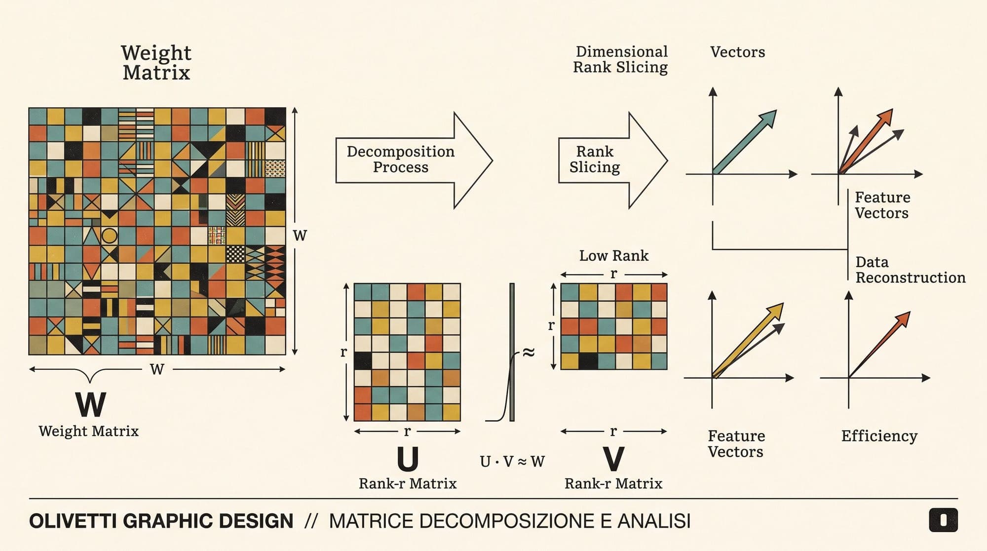
Low-Rank Adaptation (LoRA) and DoRA: Mathematical Foundations, Intrinsic Dimensionality, and Directional Weight Decomposition

Full-parameter fine-tuning of large language models presents prohibitive memory requirements during training. Standard full fine-tuning requires updating every weight matrix in a model, demanding storage not only for the model parameters themselves, but also for activation tensors, backward gradients, and first- and second-moment optimizer states. For a 70-billion-parameter model in 16-bit floating point precision, 16-bit AdamW optimizer states alone consume 1.12 TB of GPU VRAM (16 bytes per parameter: 2 bytes FP16 weight, 2 bytes FP16 gradient, 4 bytes FP32 master weight, 4 bytes FP32 momentum, and 4 bytes FP32 variance).

Parameter-Efficient Fine-Tuning (PEFT) addresses this constraint by freezing the base model parameters and updating a small fraction of specialized adapter parameters. Among PEFT methodologies, Low-Rank Adaptation (LoRA, Hu et al., 2021) and Weight-Decomposed Low-Rank Adaptation (DoRA, Liu et al., 2024) have become foundational standards.

This post details the mathematical foundations of low-rank parameterization, analyzes the intrinsic dimensionality hypothesis that justifies rank reduction, derives the gradient dynamics and normalization projections of DoRA, and examines how directional weight decomposition bridges the performance gap between low-rank adapters and full-parameter fine-tuning.

1. Theoretical Foundations: Intrinsic Dimensionality

The mathematical justification for parameter-efficient adaptation originates in the intrinsic dimensionality hypothesis of neural network optimization (Li et al., 2018; Aghajanyan et al., 2020).

A model with $D$ parameters occupies an ambient parameter space $\mathbb{R}^D$. When fine-tuning on a downstream objective $\mathcal{L}$, parameter updates $\Delta \theta \in \mathbb{R}^D$ are optimized on an empirical loss surface. The intrinsic dimension $d_{\text{intrinsic}}$ is defined as the minimum subspace dimension $d \ll D$ required to find a solution achieving at least $(1 - \epsilon)$ of the optimal objective value obtained via full parameter optimization:

$$d_{\text{intrinsic}}(\epsilon) = \min \left\{ d \in \mathbb{N} \mid \min_{\theta \in \mathbb{R}^d} \mathcal{L}(\theta_0 + P \theta) \le (1 + \epsilon) \mathcal{L}(\theta^*) \right\}$$

where $\theta_0 \in \mathbb{R}^D$ represents the frozen pre-trained weights, $P \in \mathbb{R}^{D \times d}$ is a fixed projection matrix (often drawn randomly from a Gaussian distribution), and $\theta^* \in \mathbb{R}^D$ is the unconstrained optimum.

Aghajanyan et al. (2020) demonstrated two empirical phenomena across pre-trained language models:

1. Pre-training compresses the intrinsic dimension of downstream task adaptation by orders of magnitude compared to training from random initialization.
2. Larger pre-trained base models exhibit progressively smaller intrinsic dimensions for identical downstream tasks. As model capacity $D$ scales into billions of parameters, task-specific adaptation trajectories reside on low-dimensional manifolds with $d_{\text{intrinsic}} \ll D$.

Because task adaptation operates within a low-dimensional intrinsic manifold, weight update matrices $\Delta W$ for individual linear projections possess a low intrinsic rank, enabling low-rank matrix factorization.

2. Low-Rank Adaptation (LoRA)

Mathematical Formulation

Let $W_0 \in \mathbb{R}^{d \times k}$ denote a frozen pre-trained weight matrix in a linear or attention projection layer. For an input vector $x \in \mathbb{R}^k$, the unmodified forward pass computes:

$$h = W_0 x$$

LoRA parameterizes the accumulated task-specific weight update $\Delta W \in \mathbb{R}^{d \times k}$ through a low-rank matrix decomposition:

$$\Delta W = \frac{\alpha}{r} B A$$

where $B \in \mathbb{R}^{d \times r}$ and $A \in \mathbb{R}^{r \times k}$, with rank $r \ll \min(d, k)$. The scalar $\alpha \in \mathbb{R}^+$ is a constant scaling hyperparameter.

The modified forward pass computes:

$$h = W_0 x + \Delta W x = W_0 x + \frac{\alpha}{r} B A x$$

Input x (dimension k)
   │
   ├───► [Frozen Base Weight W0 (d x k)] ──────────────────► h_base
   │                                                            │
   └───► [Trainable Down-Projection A (r x k)]                  ▼
              │                                              [ + ] ──► Output h (dimension d)
              ▼                                                 ▲
         [Trainable Up-Projection B (d x r)]                    │
              │                                                 │
              └──────► [Scaling Factor: alpha / r] ─────────────┘

Initialization Mechanics

To ensure that the adapter introduces zero perturbation to the pre-trained model outputs at step zero of training, the factor matrices are initialized asymmetrically:

$$A \sim \mathcal{N}\left(0, \sigma^2\right) \quad \text{or} \quad A \sim \mathcal{U}\left(-\sqrt{\frac{1}{k}}, \sqrt{\frac{1}{k}}\right)$$

$$B = 0$$

Because $B = 0$ at initialization:

$$\Delta W_{t=0} = \frac{\alpha}{r} (0) A = 0 \implies h_{t=0} = W_0 x + 0 = W_0 x$$

This preserves exact base model behavior at the start of fine-tuning, eliminating optimization instability that would otherwise occur from uncalibrated random additive transformations.

The Role of the Scaling Factor $\frac{\alpha}{r}$

The scalar hyperparameter $\alpha$ establishes a constant scaling magnitude. When adjusting the adapter rank $r$ across experimental sweeps (for example, comparing $r=4$, $r=16$, and $r=64$), the factor $\frac{\alpha}{r}$ normalizes the magnitude of the product $B A$.

Because the initial gradient variance scales with the inner rank dimension $r$, dividing by $r$ maintains stable gradient magnitudes when increasing rank, allowing practitioners to change $r$ without re-tuning the learning rate schedule. In common practice, $\alpha$ is often set to $2r$ or $r$, making the scaling factor equal to 2 or 1.

Memory Economics and Optimizer Footprint

In full parameter fine-tuning with AdamW, memory consumption is dominated by optimizer states:

| Component | Precision | Bytes per Parameter | Formula | | :--- | :--- | :--- | :--- | | Model Weights | FP16 / BF16 | 2 bytes | $2 \times D$ | | Gradients | FP16 / BF16 | 2 bytes | $2 \times D$ | | Master Weights | FP32 | 4 bytes | $4 \times D$ | | Momentum ($m_t$) | FP32 | 4 bytes | $4 \times D$ | | Variance ($v_t$) | FP32 | 4 bytes | $4 \times D$ | | Total per Parameter | - | 16 bytes | $16 \times D$ |

When applying LoRA with rank $r=8$ to a base weight $W_0 \in \mathbb{R}^{4096 \times 4096}$:

• Base weight parameters: $4096 \times 4096 = 16,777,216$ parameters (frozen; zero optimizer states).
• LoRA parameters: $(4096 \times 8) + (8 \times 4096) = 65,536$ parameters (0.39% of the layer).
• Trainable optimizer footprint drops from 268.4 MB down to 1.05 MB for that single layer.

Across a complete transformer, LoRA reduces active training memory requirements by up to 75% compared to full fine-tuning, while enabling training on consumer GPUs without activation offloading.

Zero-Latency Inference Merging

During serving, LoRA introduces zero additional inference latency and requires no architectural modifications to the runtime inference engine. Because matrix multiplication is distributive over addition:

$$h = W_0 x + \frac{\alpha}{r} B A x = \left( W_0 + \frac{\alpha}{r} B A \right) x = W_{\text{merged}} x$$

Before deploying to production, the low-rank delta is explicitly computed and added into the base weights:

$$W_{\text{merged}} = W_0 + \frac{\alpha}{r} B A$$

For multi-tenant applications serving thousands of task-specific adapters on a single shared base model, systems like S-LoRA (Sheng et al., 2023) and Punica (Chen et al., 2023) keep $W_0$ in base GPU memory while routing batch tokens through unified batched GEMM kernels ($B_i A_i x$), swapping adapters dynamically with minimal compute overhead.

3. Weight Decomposition Analysis: Why LoRA Diverges from Full Fine-Tuning

Despite its parameter efficiency, standard LoRA frequently exhibits an empirical performance gap when compared directly to full-parameter fine-tuning on complex reasoning, coding, and instruction-following benchmarks.

Liu et al. (2024) investigated this disparity by decomposing weight updates into their geometric components: magnitude and direction.

Magnitude and Directional Decomposition

Any weight matrix $W \in \mathbb{R}^{d \times k}$ can be uniquely decomposed into a magnitude vector $m \in \mathbb{R}^{1 \times k}$ and a directional matrix $V \in \mathbb{R}^{d \times k}$:

$$W = m \odot \frac{V}{\|V\|_c}$$

where:

• $\|V\|_c = \left[ \|v_1\|_2, \|v_2\|_2, \dots, \|v_k\|_2 \right] \in \mathbb{R}^{1 \times k}$ represents the column-wise Euclidean norm of $V$.
• $\odot$ denotes column-wise element-wise multiplication (broadcasting $m$ across rows).
• $\frac{V}{\|V\|_c}$ represents the normalized directional matrix whose columns are unit vectors on the unit hypersphere $\mathbb{S}^{d-1}$.
• $m = \|W\|_c$ represents the magnitude of each column vector in $W$.

Geometric Divergence in Weight Updates

Let $\Delta m$ denote the change in weight magnitude between pre-trained weights $W_0$ and adapted weights $W$, and let $\Delta \theta$ denote the directional change (the cosine angle between corresponding column vectors):

$$\Delta m^j = |m^j - m_0^j|$$

$$\Delta \theta^j = \arccos \left( \frac{\langle w_0^j, w^j \rangle}{\|w_0^j\|_2 \|w^j\|_2} \right)$$

where $w_0^j$ and $w^j$ denote the $j$-th column vectors of $W_0$ and $W$, respectively.

Empirical analysis reveals fundamental differences in the optimization trajectories of Full Fine-Tuning (FT) versus standard LoRA:

1. Full Fine-Tuning (FT): Shows flexible, decoupled optimization dynamics. Magnitude adjustments $\Delta m$ and directional shifts $\Delta \theta$ exhibit diverse, non-linear relationships with subtle negative correlation across layers. FT can adjust direction significantly while keeping magnitude stable, or scale magnitude while preserving orientation.
2. LoRA: In standard LoRA, $W = W_0 + \Delta W$. Because $\Delta W$ is directly added without directional normalization, magnitude changes and directional changes are coupled linearly:

$$\Delta m^j \propto \Delta \theta^j$$

In LoRA, making a large directional adjustment unavoidably increases the column norm, while small magnitude changes restrict the directional search space. This coupled constraint restricts the optimization trajectory, limiting the expressive capacity of low-rank updates.

4. Weight-Decomposed Low-Rank Adaptation (DoRA)

To resolve this limitation, Liu et al. (2024) introduced Weight-Decomposed Low-Rank Adaptation (DoRA). DoRA re-parameterizes the weight matrix by explicitly decoupling magnitude and direction, applying low-rank adaptation exclusively to the directional component while learning a separate magnitude vector.

Mathematical Formulation

DoRA parameterizes the adapted weight matrix $W \in \mathbb{R}^{d \times k}$ as:

$$W = m \odot \frac{V}{\|V\|_c} = m \odot \frac{W_0 + \Delta W}{\|W_0 + \Delta W\|_c} = m \odot \frac{W_0 + \frac{\alpha}{r} B A}{\|W_0 + \frac{\alpha}{r} B A\|_c}$$

where:

• $W_0 \in \mathbb{R}^{d \times k}$ is the frozen pre-trained weight matrix.
• $B \in \mathbb{R}^{d \times r}$ and $A \in \mathbb{R}^{r \times k}$ are trainable low-rank matrices, initialized with $B = 0$ and $A \sim \mathcal{N}(0, \sigma^2)$.
• $m \in \mathbb{R}^{1 \times k}$ is a trainable magnitude vector, initialized to the column norms of the pre-trained weight: $m = \|W_0\|_c$.
• $\Delta W = \frac{\alpha}{r} B A$ is the low-rank directional update.

At step zero ($t = 0$): $$\Delta W = 0 \implies V = W_0 \implies \frac{V}{\|V\|_c} = \frac{W_0}{\|W_0\|_c}$$

$$W_{t=0} = \|W_0\|_c \odot \frac{W_0}{\|W_0\|_c} = W_0$$

DoRA preserves the exact identity mapping at initialization while completely uncoupling magnitude learning from directional updates.

Forward Pass Computation

For an input activation tensor $X \in \mathbb{R}^{b \times k}$ (with batch size and sequence length collapsed into dimension $b$), the forward output $Y \in \mathbb{R}^{b \times d}$ is computed as:

$$Y = X W^T = X \left( m \odot \frac{W_0 + \frac{\alpha}{r} B A}{\|W_0 + \frac{\alpha}{r} B A\|_c} \right)^T$$

To maintain training efficiency without explicitly materializing the full dense matrix $W \in \mathbb{R}^{d \times k}$ on every forward step, the computation can be structured around normalized base projections and normalized adapter pathways:

$$V = W_0 + \frac{\alpha}{r} B A$$

$$\tilde{V} = \frac{V}{\|V\|_c}$$

$$Y = \left( X \tilde{V}^T \right) \odot m$$

Exact Gradient Derivations

The optimization dynamics of DoRA are governed by the gradients with respect to the magnitude vector $m$ and the low-rank directional factors $A$ and $B$.

Let $\mathcal{L}$ be the scalar objective loss, and let $G = \frac{\partial \mathcal{L}}{\partial W} \in \mathbb{R}^{d \times k}$ denote the upstream gradient with respect to the reconstructed weight $W$.

Gradient with respect to Magnitude $m$

Using the chain rule:

$$\frac{\partial \mathcal{L}}{\partial m^j} = \sum_{i=1}^d \frac{\partial \mathcal{L}}{\partial W_{ij}} \frac{\partial W_{ij}}{\partial m^j} = \sum_{i=1}^d G_{ij} \frac{V_{ij}}{\|v_j\|_2} = \left\langle G_{:, j}, \frac{v_j}{\|v_j\|_2} \right\rangle$$

In vector notation across all columns:

$$\nabla_m \mathcal{L} = \sum_{\text{rows}} \left( G \odot \frac{V}{\|V\|_c} \right) \in \mathbb{R}^{1 \times k}$$

The gradient of $m$ is simply the projection of the gradient $G$ onto the current directional unit vector.

Gradient with respect to Directional Matrix $V$

For a single column $v_j \in \mathbb{R}^d$ and corresponding weight column $w_j = m^j \frac{v_j}{\|v_j\|_2}$:

$$\frac{\partial w_j}{\partial v_j} = \frac{m^j}{\|v_j\|_2} \left( I - \frac{v_j v_j^T}{\|v_j\|_2^2} \right)$$

Applying the chain rule with upstream gradient $g_j = G_{:, j} \in \mathbb{R}^d$:

$$\nabla_{v_j} \mathcal{L} = \left( \frac{\partial w_j}{\partial v_j} \right)^T g_j = \frac{m^j}{\|v_j\|_2} \left( g_j - \frac{\langle g_j, v_j \rangle}{\|v_j\|_2^2} v_j \right) = \frac{m^j}{\|v_j\|_2} P_{v_j}^\perp g_j$$

where:

$$P_{v_j}^\perp = \left( I - \frac{v_j v_j^T}{\|v_j\|_2^2} \right)$$

$P_{v_j}^\perp$ is the orthogonal projection operator onto the tangent space of the unit sphere at $\frac{v_j}{\|v_j\|_2}$.

This formulation provides two structural properties:

1. Gradient Orthogonality: The directional gradient $\nabla_{v_j} \mathcal{L}$ is orthogonal to $v_j$ ($\langle \nabla_{v_j} \mathcal{L}, v_j \rangle = 0$), ensuring that directional updates rotate the weight vector along the sphere without altering its norm.
2. Self-Stabilizing Scale Invariance: The gradient magnitude is scaled inversely by $\|v_j\|_2$. If the norm of $V$ grows large during optimization, directional gradients are automatically scaled down, stabilizing training dynamics without requiring explicit weight clipping.

From $\nabla_V \mathcal{L}$, the gradients with respect to the low-rank factors $A$ and $B$ follow via standard matrix calculus:

$$\nabla_B \mathcal{L} = \frac{\alpha}{r} \left( \nabla_V \mathcal{L} \right) A^T \in \mathbb{R}^{d \times r}$$

$$\nabla_A \mathcal{L} = \frac{\alpha}{r} B^T \left( \nabla_V \mathcal{L} \right) \in \mathbb{R}^{r \times k}$$

Inference Merging in DoRA

Like LoRA, DoRA incurs zero extra latency during inference deployment. The merged weight matrix $W_{\text{merged}}$ is computed offline prior to deployment:

$$W_{\text{merged}} = m \odot \frac{W_0 + \frac{\alpha}{r} B A}{\|W_0 + \frac{\alpha}{r} B A\|_c} \in \mathbb{R}^{d \times k}$$

Once $W_{\text{merged}}$ is evaluated, it replaces the base weight $W_0$ in the standard inference runtime model file.

5. Architectural Target Modules, Rank Dynamics, and Quantization

Target Module Selection

In standard transformer architectures (such as LLaMA, Mistral, and Qwen), linear projections exist within both the multi-head self-attention (MHA) and feed-forward network (FFN/MLP) blocks:

• Attention Projections: Query ($W_q$), Key ($W_k$), Value ($W_v$), and Output ($W_o$).
• Feed-Forward Projections: Gate ($W_{\text{gate}}$), Up ($W_{\text{up}}$), and Down ($W_{\text{down}}$) in SwiGLU architectures.

Early LoRA implementations (Hu et al., 2021) applied adapters solely to $W_q$ and $W_v$. Subsequent empirical evaluations (Dettmers et al., 2023) demonstrated that applying low-rank adapters across all linear layers ($W_q, W_k, W_v, W_o, W_{\text{gate}}, W_{\text{up}}, W_{\text{down}}$) with a smaller rank $r$ (e.g., $r=8$ or $r=16$) consistently outperforms allocating a large rank (e.g., $r=64$) to attention layers alone.

Transformer Layer
├── Multi-Head Attention Block
│   ├── W_q (LoRA / DoRA target)
│   ├── W_k (LoRA / DoRA target)
│   ├── W_v (LoRA / DoRA target)
│   └── W_o (LoRA / DoRA target)
└── SwiGLU MLP Block
    ├── W_gate (LoRA / DoRA target)
    ├── W_up   (LoRA / DoRA target)
    └── W_down (LoRA / DoRA target)

Singular Spectrum and Effective Rank Analysis

When training low-rank factor matrices $B A \in \mathbb{R}^{d \times k}$, singular value decomposition (SVD) of the learned update $\Delta W = U \Sigma V^T$ illuminates the rank distribution:

$$\Sigma = \text{diag}(\sigma_1, \sigma_2, \dots, \sigma_r), \quad \sigma_1 \ge \sigma_2 \ge \dots \ge \sigma_r \ge 0$$

The effective rank $r_{\text{eff}}$ of the learned update matrix can be quantified via the entropy of the normalized singular value distribution $p_i = \frac{\sigma_i}{\sum_{j=1}^r \sigma_j}$:

$$r_{\text{eff}} = \exp \left( -\sum_{i=1}^r p_i \ln p_i \right)$$

Empirical observations from SVD spectrum studies show:

1. Rank Saturation in LoRA: Even when nominal rank is configured to $r=64$, the top 4 to 8 singular values often capture over 90% of the spectral energy $\sum \sigma_i^2$, indicating that standard LoRA struggles to utilize higher rank dimensions effectively due to magnitude-direction coupling.
2. Spectral Diversity in DoRA: By isolating magnitude updates into $m$, DoRA maintains a broader, flatter singular value spectrum across $B A$, achieving higher effective rank $r_{\text{eff}}$ for identical nominal rank settings.

QLoRA Integration (4-Bit Quantized Base Weights)

To minimize training memory, LoRA and DoRA can be paired with QLoRA (Dettmers et al., 2023):

• NF4 (NormalFloat 4): An information-theoretically optimal quantile quantization data type for normally distributed neural network weights.
• Double Quantization (DQ): Quantizing the quantization constants themselves, saving approximately 0.37 bits per parameter (reducing footprint from 0.5 bytes to 0.128 bytes per parameter for quantization constants).
• Paged Optimizers: Utilizing CUDA Unified Memory to automatically page 32-bit AdamW optimizer states between GPU VRAM and CPU system RAM during memory spikes.

Under QLoRA + DoRA (QDoRA):

• Base weights $W_0$ reside in frozen 4-bit NF4 representation ($0.5$ bytes per parameter).
• On the forward pass, $W_0$ is dequantized on-the-fly to BF16, added to $\frac{\alpha}{r} B A$, normalized by column norms, and scaled by $m$.
• Backward gradients are calculated only with respect to FP16/BF16 adapter parameters $A, B$ and vector $m$.

This allows fine-tuning a 70B parameter model on a single 48 GB GPU or two 24 GB consumer GPUs.

6. PyTorch Reference Implementation

The following self-contained PyTorch module demonstrates the exact structural formulation of a Weight-Decomposed Low-Rank Adaptation (DoRA) linear layer:

import torch
import torch.nn as nn
import torch.nn.functional as F
import math

class DoRALinear(nn.Module):
    def __init__(
        self,
        in_features: int,
        out_features: int,
        rank: int = 8,
        alpha: float = 16.0,
        dropout: float = 0.0,
        bias: bool = False
    ):
        super().__init__()
        self.in_features = in_features
        self.out_features = out_features
        self.rank = rank
        self.alpha = alpha
        self.scaling = alpha / rank

        # Frozen base pre-trained linear layer
        self.base_layer = nn.Linear(in_features, out_features, bias=bias)
        self.base_layer.weight.requires_grad = False
        if bias:
            self.base_layer.bias.requires_grad = False

        if rank > 0:
            # Low-rank directional adapters
            self.lora_A = nn.Parameter(torch.empty(rank, in_features))
            self.lora_B = nn.Parameter(torch.zeros(out_features, rank))
            
            # Learnable magnitude parameter vector m (per output channel/row)
            # In PyTorch Linear, weight is (out_features, in_features).
            # The directional norm is computed across in_features (dim=1).
            with torch.no_grad():
                init_norm = torch.linalg.norm(self.base_layer.weight, dim=1, keepdim=True)
            self.magnitude = nn.Parameter(init_norm.clone())

            self.dropout = nn.Dropout(p=dropout) if dropout > 0.0 else nn.Identity()
            self._reset_lora_parameters()
        else:
            self.lora_A = None
            self.lora_B = None
            self.magnitude = None

    def _reset_lora_parameters(self):
        # Kaiming uniform initialization for A, zero for B
        nn.init.kaiming_uniform_(self.lora_A, a=math.sqrt(5))
        nn.init.zeros_(self.lora_B)

    def forward(self, x: torch.Tensor) -> torch.Tensor:
        if self.rank == 0:
            return self.base_layer(x)

        # 1. Compute directional weight matrix V = W0 + (alpha / r) * B @ A
        # Base weight shape: (out_features, in_features)
        lora_weight = (self.lora_B @ self.lora_A) * self.scaling
        V = self.base_layer.weight + lora_weight

        # 2. Compute directional column/row norm ||V||
        # Normalizing each output channel's weight vector across in_features
        V_norm = torch.linalg.norm(V, dim=1, keepdim=True)

        # 3. Form unit directional matrix and scale by magnitude vector m
        adapted_weight = self.magnitude * (V / (V_norm + 1e-8))

        # 4. Standard linear forward pass with adapted weight
        bias = self.base_layer.bias if self.base_layer.bias is not None else None
        return F.linear(x, adapted_weight, bias)

    @torch.no_grad()
    def merge_weights(self):
        """Merges DoRA parameters permanently into base_layer for zero-overhead inference."""
        if self.rank > 0:
            lora_weight = (self.lora_B @ self.lora_A) * self.scaling
            V = self.base_layer.weight + lora_weight
            V_norm = torch.linalg.norm(V, dim=1, keepdim=True)
            merged = self.magnitude * (V / (V_norm + 1e-8))
            self.base_layer.weight.copy_(merged)
            self.rank = 0
            del self.lora_A, self.lora_B, self.magnitude

7. Empirical Benchmarks and Comparative Analysis

Extensive empirical evaluations across open-weight language and multimodal architectures demonstrate how DoRA consistently outperforms standard LoRA while matching or exceeding Full Fine-Tuning across diverse domains.

Commonsense Reasoning (LLaMA-7B and LLaMA-13B)

On standard commonsense reasoning benchmarks (incorporating BoolQ, PIQA, SIQA, HellaSwag, WinoGrande, ARC-Easy, ARC-Challenge, and OpenBookQA), the comparative accuracy profiles reported by Liu et al. (2024) demonstrate clear performance gains:

| Method | Base Model | Trainable Params | Average Accuracy (%) | | :--- | :--- | :--- | :--- | | Full Fine-Tuning (FT) | LLaMA-7B | 6.7B (100%) | 78.2 | | LoRA ($r=8$) | LLaMA-7B | 18.0M (0.27%) | 77.4 | | DoRA ($r=8$) | LLaMA-7B | 18.2M (0.27%) | 78.4 | | LoRA ($r=16$) | LLaMA-7B | 36.0M (0.54%) | 77.9 | | DoRA ($r=16$) | LLaMA-7B | 36.2M (0.54%) | 78.7 | | Full Fine-Tuning (FT) | LLaMA-13B | 13.0B (100%) | 80.0 | | LoRA ($r=8$) | LLaMA-13B | 29.5M (0.23%) | 79.2 | | DoRA ($r=8$) | LLaMA-13B | 29.8M (0.23%) | 80.3 |

Key finding: DoRA with rank $r=8$ outperforms LoRA with rank $r=16$ while using half the low-rank parameters, surpassing full fine-tuning performance on commonsense reasoning.

Visual Instruction Tuning (LLaVA-1.5-7B)

On vision-language tasks evaluating visual reasoning, optical character recognition, and spatial grounding (incorporating VQA-v2, GQA, VizWiz, SQA, and TextVQA):

| Method | Base Model | VQA-v2 | GQA | VizWiz | SQA | TextVQA | Average | | :--- | :--- | :--- | :--- | :--- | :--- | :--- | :--- | | Full Fine-Tuning | LLaVA-1.5-7B | 78.5 | 62.0 | 50.0 | 66.8 | 58.2 | 63.1 | | LoRA ($r=64$) | LLaVA-1.5-7B | 79.1 | 63.0 | 48.7 | 68.4 | 57.5 | 63.3 | | DoRA ($r=64$) | LLaVA-1.5-7B | 79.6 | 63.7 | 50.6 | 69.8 | 58.6 | 64.5 |

Structural Comparison Summary

| Feature | Full Fine-Tuning (FT) | LoRA (Hu et al., 2021) | DoRA (Liu et al., 2024) | | :--- | :--- | :--- | :--- | | Trainable Parameters | 100% | 0.1% to 1.0% | 0.1% to 1.0% + magnitude vectors | | Optimizer Memory | 16 bytes / param | Scaled to adapter rank only | Scaled to adapter rank only | | Magnitude-Direction Dynamics | Decoupled | Proportional / Linearly Coupled | Strictly Decoupled | | Training Throughput | Baseline (1.0x) | ~1.15x (less memory, faster step) | ~1.05x to 1.10x (normalization step) | | Inference Latency Overhead | Zero (native base) | Zero (merged $W_0 + \Delta W$) | Zero (merged $m \odot \frac{V}{\|V\|}$) | | Multi-Tenant Adapter Swapping | Unsupported | Supported (dynamic S-LoRA) | Supported (dynamic routing) |

8. Summary and Architectural Takeaways

Parameter-efficient fine-tuning has evolved from an empirical heuristic to a geometrically rigorous discipline. The progression from full fine-tuning to LoRA and DoRA illustrates three architectural principles:

1. Intrinsic Dimension Minimization: Pre-trained representations constrain task adaptation to low-dimensional parameter sub-manifolds, enabling matrix factorizations with rank $r \ll d$.
2. Directional Decoupling: LoRA's limitation stems from coupling weight magnitude updates to directional shifts. By decomposing weights into magnitude vectors and directional unit matrices, DoRA mirrors the gradient dynamics of full fine-tuning.
3. Zero Inference Penalty: Both LoRA and DoRA allow offline weight re-parameterization, merging adapter updates directly into base models to deliver parameter-efficient adaptation with zero runtime inference overhead.

Sources

• LoRA: Low-Rank Adaptation of Large Language Models (Hu et al., 2021)
• DoRA: Weight-Decomposed Low-Rank Adaptation (Liu et al., 2024)
• QLoRA: Efficient Finetuning of Quantized LLMs (Dettmers et al., 2023)
• Intrinsic Dimensionality Explains the Effectiveness of Language Model Fine-Tuning (Aghajanyan et al., 2020)
• Measuring the Intrinsic Dimension of Objective Landscapes (Li et al., 2018)
• S-LoRA: Serving Thousands of Concurrent LoRA Adapters (Sheng et al., 2023)
• Punica: Multi-Tenant LoRA Serving (Chen et al., 2023)