Knowledge Distillation: Mathematical Foundations, Dark Knowledge, Soft Target Regularization, and Sequence-Level Policy Transfer

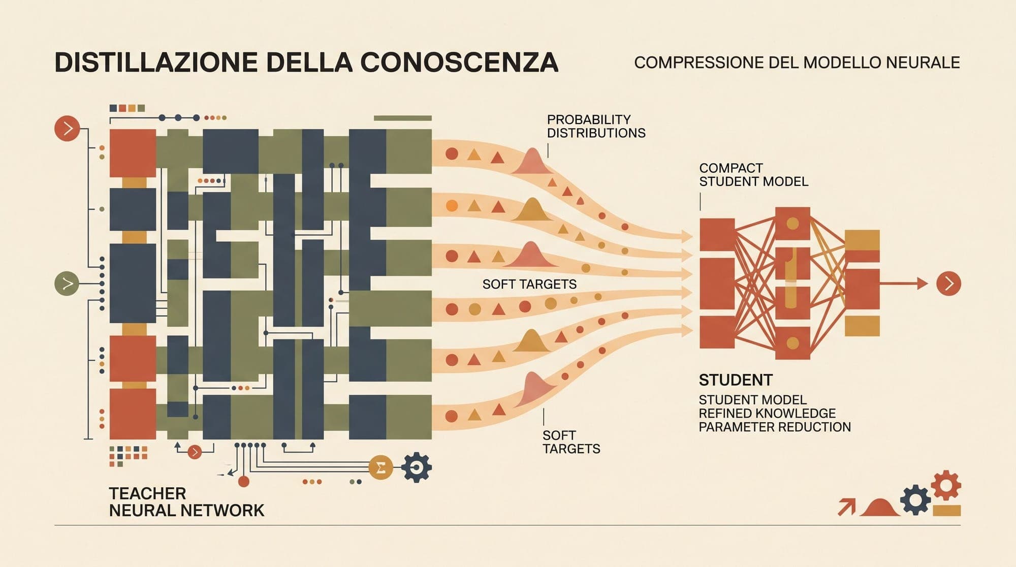
Knowledge distillation is a foundational model compression and transfer technique wherein a compact "student" neural network is trained to reproduce the functional behavior, internal representations, or output distributions of a larger, high-capacity "teacher" model or ensemble. First formalized in modern deep learning by Hinton, Vinyals, and Dean (2015), following earlier foundational work on model compression by Buciluǎ et al. (2006), distillation exploits the rich inductive biases and dark knowledge encoded within the teacher model's continuous probability outputs.

In modern large language model (LLM) pipelines, distillation serves as the primary mechanism for transferring reasoning traces, instruction-following proficiency, and domain capabilities from massive foundation models to lightweight, edge-deployable, or low-latency serving models. This guide examines the mathematical mechanics of soft target distillation, the behavior of temperature scaling, intermediate representation matching, sequence-level policy transfer, and the divergence dynamics between forward and reverse Kullback-Leibler objectives.

1. Mathematical Formulation and the "Dark Knowledge" Principle

Traditional supervised classification trains models against one-hot categorical target vectors $y \in \{0, 1\}^K$, where $K$ is the number of classes. While one-hot encoding penalizes incorrect ground-truth assignments, it provides zero gradient feedback regarding the relative structural similarity between incorrect candidate classes.

A high-capacity teacher network trained on large corpora produces a continuous logit vector $z^T \in \mathbb{R}^K$. When normalized through a softmax function, the resulting probability vector assigns small but non-zero probabilities to incorrect classes. These non-target probabilities constitute what Hinton et al. termed dark knowledge. For instance, when classifying an image of a BMW, the teacher may assign a probability of 0.85 to "BMW", 0.14 to "Audi", and $10^{-6}$ to "Garbage Truck". The relative ratio between "BMW" and "Audi" communicates geometric and structural manifold information that one-hot vectors destroy.

Standard Supervised Loss:
y_true = [0,  0,  1,  0,  0]  (One-Hot: Absolute certainty, zero inter-class geometry)

Teacher Soft Output (Dark Knowledge):
p_teacher = [0.01, 0.04, 0.78, 0.16, 0.01] (Continuous manifold: reveals class correlations)

By forcing the student network to match these soft probability distributions, the student inherits the teacher's geometric decision boundaries without requiring the same parameter volume.

2. Temperature-Scaled Softmax and the Distillation Objective

Directly applying a standard softmax function $\sigma(z_i) = \frac{\exp(z_i)}{\sum_j \exp(z_j)}$ suppresses small logits toward zero due to the exponential operator, hiding the dark knowledge. To amplify the signal in the non-target tail, a temperature hyperparameter $T > 0$ is introduced to scale the pre-activation logits prior to normalization.

For a logit vector $z$, the temperature-scaled probability for class $i$ is defined as:

$$q_i(z, T) = \frac{\exp(z_i / T)}{\sum_{j=1}^K \exp(z_j / T)}$$

As $T \to 0$, $q(z, T)$ collapses into a hard argmax (one-hot) vector. As $T \to \infty$, $q(z, T)$ approaches a uniform discrete distribution $1/K$. At intermediate values ($T \in [2, 10]$), the distribution flattens sufficiently to expose inter-class variance while preserving mode ranking.

The Complete Distillation Loss

The canonical knowledge distillation objective balances hard ground-truth supervised cross-entropy with soft teacher-matching Kullback-Leibler (KL) divergence:

$$\mathcal{L}_{KD}(\theta_S) = (1 - \alpha) \mathcal{L}_{CE}(y, q(z^S, 1)) + \alpha T^2 \mathcal{D}_{KL}\left(q(z^T, T) \parallel q(z^S, T)\right)$$

Where:

• $\theta_S$ represents the trainable parameters of the student network.
• $z^S$ and $z^T$ are the student and teacher logit vectors, respectively.
• $\alpha \in [0, 1]$ is a balancing coefficient.
• $\mathcal{L}_{CE}$ is the standard categorical cross-entropy loss against ground-truth labels $y$.
• $\mathcal{D}_{KL}(P \parallel Q) = \sum_i P_i \log(P_i / Q_i)$ is the KL divergence from student distribution $Q$ to teacher distribution $P$.
• $T^2$ is an essential gradient scaling factor.

The $T^2$ Gradient Normalization Factor

To understand why the $T^2$ multiplier is mathematically necessary, consider the gradient of the soft loss component with respect to a student logit $z_i^S$.

Let $\mathcal{L}_{soft} = \mathcal{D}_{KL}(q^T \parallel q^S) = \sum_j q_j^T \log q_j^T - \sum_j q_j^T \log q_j^S$. The partial derivative with respect to $z_i^S$ is:

$$\frac{\partial \mathcal{L}_{soft}}{\partial z_i^S} = \frac{1}{T} \left( q_i(z^S, T) - q_i(z^T, T) \right)$$

When $T$ is large relative to the magnitude of the logits, we can use the first-order Taylor expansion $\exp(x) \approx 1 + x$:

$$q_i(z, T) \approx \frac{1 + z_i / T}{K + \sum_j z_j / T} = \frac{1 + z_i / T}{K + K \bar{z} / T} \approx \frac{1}{K} \left( 1 + \frac{z_i - \bar{z}}{T} \right)$$

Where $\bar{z} = \frac{1}{K} \sum_j z_j$ is the mean logit. Substituting this approximation into the gradient expression yields:

$$\frac{\partial \mathcal{L}_{soft}}{\partial z_i^S} \approx \frac{1}{T} \left[ \frac{1}{K} \left( 1 + \frac{z_i^S - \bar{z}^S}{T} \right) - \frac{1}{K} \left( 1 + \frac{z_i^T - \bar{z}^T}{T} \right) \right] = \frac{1}{K T^2} \left( (z_i^S - \bar{z}^S) - (z_i^T - \bar{z}^T) \right)$$

Because the magnitude of the gradient scales inversely with $T^2$, failing to multiply the loss by $T^2$ causes the gradient from the teacher to vanish as temperature increases. Multiplying $\mathcal{L}_{soft}$ by $T^2$ stabilizes the effective learning rate across arbitrary temperature selections and demonstrates that high-temperature distillation is mathematically equivalent to minimizing the Mean Squared Error (MSE) between zero-mean logit vectors.

3. Intermediate Representation Matching and Feature Distillation

Matching final output distributions constrains only the terminal layer of the network. To accelerate convergence and guide the internal representational geometry of the student, intermediate feature distillation matches activations across hidden layers.

Teacher Network:   [Embedding] -> [Hidden Layer 12] -> [Hidden Layer 24] -> [Logits]
                                        |                    |                |
                                (Proj / Attention)   (Proj / Hidden)     (Soft Targets)
                                        |                    |                |
Student Network:   [Embedding] -> [Hidden Layer 3]  -> [Hidden Layer 6]  -> [Logits]

1. FitNets (Hint-Based Training)

Introduced by Romero et al. (2014), FitNets introduce intermediate "hint" layers in the teacher and "guided" layers in the student. Because the student hidden dimension $d_S$ is typically smaller than the teacher hidden dimension $d_T$, a learnable linear transformation matrix $W_r \in \mathbb{R}^{d_T \times d_S}$ projects student activations into the teacher space:

$$\mathcal{L}_{hint} = \frac{1}{2} \left\| h^T - W_r h^S \right\|_2^2$$

2. Attention Map Transfer

Zagoruyko and Komodakis (2016) demonstrated that spatial attention maps carry rich localization knowledge. For an intermediate activation tensor $A \in \mathbb{R}^{C \times H \times W}$, a 2D spatial attention map is computed by summing the absolute values across channel dimensions:

$$F_{sum}(A) = \sum_{c=1}^C |A_{c, :, :}|^p$$

The attention distillation loss minimizes the normalized $L_2$ distance between student and teacher attention maps:

$$\mathcal{L}_{AT} = \sum_{l \in \mathcal{I}} \left\| \frac{F(A_S^{(l)})}{\|F(A_S^{(l)})\|_2} - \frac{F(A_T^{(l)})}{\|F(A_T^{(l)})\|_2} \right\|_2$$

3. Relational Distillation

Rather than matching individual activations in isolation, relational knowledge distillation (Park et al., 2019) transfers structural distances and angles across mini-batch samples. If a batch contains $N$ examples, the student is trained to preserve the pairwise cosine similarity matrix and triplet angular configurations constructed by the teacher.

4. Sequence-Level Distillation in Autoregressive Language Models

Distilling autoregressive language models $P(y|x) = \prod_{t=1}^{|y|} P(y_t | y_{<t}, x)$ presents challenges absent in standard classification. A naive token-level cross-entropy loss against teacher token distributions treats each decoding step independently, ignoring sequence-level dependencies.

Word-Level KD vs. Sequence-Level KD (SeqKD)

Kim and Rush (2016) formalized the distinction between word-level and sequence-level distillation for sequence-to-sequence models:

• Word-Level Distillation: The student is trained on ground-truth target tokens using teacher token distributions $P_T(y_t | y_{<t}^, x)$ conditioned on ground-truth prefixes $y_{<t}^$. This suffers from exposure bias because during inference, the student conditions on its own prior generations rather than ground-truth tokens.
• Sequence-Level Distillation (SeqKD): The teacher model generates a complete sequence using beam search decoding:

$$\hat{y} = \arg\max_y P_T(y | x)$$ The student is then trained via standard supervised maximum likelihood directly on the teacher-generated outputs $(x, \hat{y})$. SeqKD approximates matching the entire sequence-level distribution $P_T(Y|X)$ by replacing the intractable sum over all possible sequences with the mode of the teacher's distribution.

5. Forward KL vs. Reverse KL: Mode Covering vs. Mode Seeking

In LLM distillation, the mathematical choice of divergence metric fundamentally dictates the student model's generative behavior and error profile.

Target Teacher Distribution: Bimodal (Two distinct valid responses)
          /\          /\
_________/  \________/  \_________

Forward KL (Mode-Covering / Zero-Avoiding):
Student stretches across both modes, assigning non-zero mass to low-density valleys (hallucinations).
        /----------------\
_______/                  \_______

Reverse KL (Mode-Seeking / Zero-Forcing):
Student locks onto a single sharp mode, producing precise, coherent outputs.
          /\
_________/  \_____________________

Forward KL ($\mathcal{D}_{KL}(P_T \parallel P_S)$)

The standard distillation objective computes:

$$\mathcal{D}_{KL}(P_T \parallel P_S) = \mathbb{E}_{y \sim P_T} \left[ \log \frac{P_T(y|x)}{P_S(y|x)} \right] = \sum_y P_T(y|x) \log P_T(y|x) - \sum_y P_T(y|x) \log P_S(y|x)$$

Forward KL is zero-avoiding (mode-covering). If $P_T(y|x) > 0$, the student must ensure $P_S(y|x) > 0$ to prevent $\log(P_T / P_S)$ from approaching infinity. Consequently, a capacity-limited student tries to cover all modes of the teacher, averaging disparate outputs and placing probability mass in low-probability regions between modes. In text generation, this manifests as blurs, inconsistent syntax, and hallucinations.

Reverse KL ($\mathcal{D}_{KL}(P_S \parallel P_T)$)

Conversely, reverse KL computes:

$$\mathcal{D}_{KL}(P_S \parallel P_T) = \mathbb{E}_{y \sim P_S} \left[ \log \frac{P_S(y|x)}{P_T(y|x)} \right] = \sum_y P_S(y|x) \log P_S(y|x) - \sum_y P_S(y|x) \log P_T(y|x)$$

Reverse KL is zero-forcing (mode-seeking). If $P_T(y|x) \approx 0$, the student is heavily penalized if $P_S(y|x) > 0$. The student minimizes the objective by setting $P_S(y|x) = 0$ wherever the teacher has low probability, safely concentrating its limited capacity on a subset of the teacher's primary modes.

MiniLLM and Policy Gradient Optimization

Because sampling from $y \sim P_S$ in reverse KL prevents standard backpropagation through discrete token selections, Gu et al. (2023) formulated MiniLLM, which optimizes reverse KL using reinforcement learning policy gradients:

$$\nabla_{\theta_S} \mathcal{D}_{KL}(P_S \parallel P_T) = \mathbb{E}_{y \sim P_S} \left[ \nabla_{\theta_S} \log P_S(y|x) \left( \log \frac{P_S(y|x)}{P_T(y|x)} - 1 \right) \right]$$

By utilizing single-step trajectory rollouts and reward baselines, MiniLLM enables stable on-policy student distillation, eliminating the tail-blurring artifacts of forward KL.

6. Modern LLM Distillation: Reasoning and Step-Level Trajectories

In reasoning-focused architectures (such as mathematical reasoning, program synthesis, and multi-turn planning), distilling raw token distributions is insufficient. Modern workflows combine chain-of-thought (CoT) synthesis with verification filtering:

1. Trajectory Sampling: A frontier model generates $N$ independent chain-of-thought solutions for each problem: $\tau = (x, r_1, r_2, \dots, r_k, y)$.
2. Outcome and Process Verification: Trajectories are validated against verifiable execution environments (unit tests, math solvers) or Process Reward Models (PRMs). Incorrect paths are rejected.
3. Step-Level Credit Assignment: Distillation is applied across verified rationales, training the compact student to replicate intermediate deductions prior to emitting final solutions.
4. Student On-Policy Exploration: The student generates its own trajectories, and the teacher evaluates step-level transitions, providing fine-grained advantage signals via RL algorithms such as PPO or GRPO.

7. Comparative Analysis of Distillation Paradigms

• Response-Based Distillation (Hinton et al.): Optimizes $\mathcal{D}_{KL}(q^T \parallel q^S)$ on output logits. Advantages: simple implementation, architecture-agnostic. Primary limitation: ignores internal representation geometry and requires careful tuning of $T$.
• Feature-Based Distillation (FitNets): Optimizes $\|h^T - W_r h^S\|_2^2$ on hidden activations. Advantages: accelerates convergence and structures latent spaces. Primary limitation: requires intermediate dimension projection matrices and increases memory during training.
• Attention Transfer: Optimizes $\|F(A_T) - F(A_S)\|_2$ across multi-head attention maps. Advantages: preserves attention focus and inter-token routing. Primary limitation: sensitive to architectural mismatch in head counts and layer depths.
• Sequence-Level Distillation (SeqKD): Optimizes $\mathcal{L}_{CE}(y_{beam}^T, z^S)$ on complete autoregressive generations. Advantages: directly mitigates exposure bias. Primary limitation: risks mode collapse on ambiguous or open-ended prompts.
• Reverse-KL On-Policy Distillation (MiniLLM): Optimizes $\mathcal{D}_{KL}(P_S \parallel P_T)$ on student rollouts via policy gradients. Advantages: strictly mode-seeking, eliminates hallucination in zero-probability regions. Primary limitation: higher training variance and requires RL optimization scaffolding.

Sources

• Distilling the Knowledge in a Neural Network (Hinton, Vinyals, Dean, 2015)
• Model Compression (Buciluǎ, Caruana, Niculescu-Mizil, 2006)
• FitNets: Hints for Thin Deep Nets (Romero et al., 2014)
• Paying More Attention to Attention: Improving the Performance of Convolutional Neural Networks via Attention Transfer (Zagoruyko & Komodakis, 2016)
• Relational Knowledge Distillation (Park et al., 2019)
• Sequence-Level Knowledge Distillation (Kim & Rush, 2016)
• Knowledge Distillation of Large Language Models (Gu et al., 2023)
• A Survey on Knowledge Distillation of Large Language Models (Xu et al., 2024)