Induction Heads: Mathematical Foundations, Two-Layer Circuit Composition, and the Emergence of In-Context Learning in Transformers

One of the defining capabilities of modern autoregressive large language models is in-context learning: the ability to infer rules, adapt to task formats, and execute complex few-shot instructions purely from prompt context without updating neural network weights. For years, in-context learning was treated as an enigmatic, emergent property of large-scale autoregressive pre-training.

However, mechanistic interpretability research spearheaded by Anthropic (most notably in the landmark papers by Elhage et al. (2021) and Olsson et al. (2022)) demonstrated that in-context learning is driven by concrete, identifiable algorithmic sub-circuits known as induction heads.

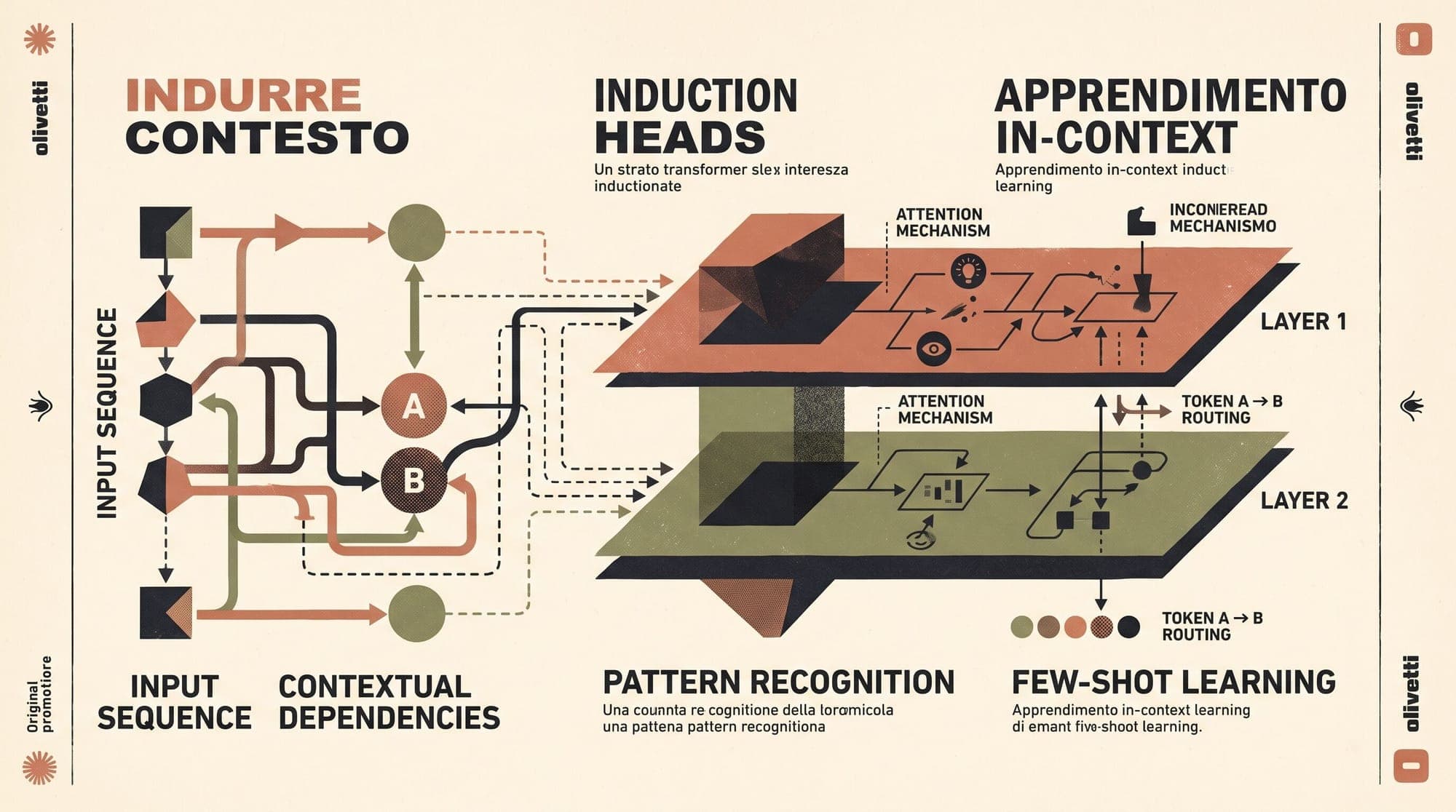
Induction heads operate across transformer attention layers via inter-head composition. By combining a "previous-token head" in an early layer with an "induction head" in a downstream layer, the transformer implements a general pattern-matching and copying algorithm: if pattern $[A][B]$ appeared previously in the context, and the current token is $[A]$, the circuit attends back to $[B]$ and boosts its probability as the next token.

Moreover, induction heads do not form gradually throughout pre-training. They crystallize during a sharp, macroscopic phase transition early in training, directly coinciding with a steep reduction in in-context loss across model scales.

Understanding the mathematical mechanics, matrix factorization, and circuit dynamics of induction heads provides fundamental insight into how transformer architectures transition from simple n-gram memorization to general algorithmic reasoning.

1. The Transformer Circuit Decomposition Framework

To analyze induction heads rigorously, we adopt the mathematical framework of transformer circuits formulated by Elhage et al. (2021).

The Residual Stream as a Linear Communication Bus

In a standard decoder-only transformer with $L$ layers, hidden dimension $d_{\text{model}}$, and $H$ attention heads per layer, the central backbone is the residual stream. For a sequence of $N$ input tokens $t = (t_1, t_2, \dots, t_N)$, the initial representations are formed by token and positional embeddings:

$$x_i^{(0)} = W_E t_i + W_{\text{pos}}(i), \quad x_i^{(0)} \in \mathbb{R}^{d_{\text{model}}}$$

Each attention layer and feed-forward network (MLP) reads from the residual stream and adds its output back into the stream via residual connections:

$$x_i^{(\ell)} = x_i^{(\ell-1)} + \sum_{h=1}^H \text{Attn}^{(\ell, h)}(x^{(\ell-1)})_i + \text{MLP}^{(\ell)}(x^{(\ell-1)})_i$$

Finally, the output logits for predicting token $t_{N+1}$ are computed by applying the unembedding matrix $W_U \in \mathbb{R}^{V \times d_{\text{model}}}$:

$$\text{logits}_{N+1} = W_U x_N^{(L)}$$

Because residual connections are additive, the residual stream acts as a linear communication channel where individual attention heads write vectors into specific subspaces without overwriting existing representations.

Factorizing Attention: QK and OV Circuits

For an individual attention head $h$ in layer $\ell$, parameterized by query matrix $W_Q \in \mathbb{R}^{d_{\text{head}} \times d_{\text{model}}}$, key matrix $W_K \in \mathbb{R}^{d_{\text{head}} \times d_{\text{model}}}$, value matrix $W_V \in \mathbb{R}^{d_{\text{head}} \times d_{\text{model}}}$, and output projection $W_O \in \mathbb{R}^{d_{\text{model}} \times d_{\text{head}}}$, the head's computation factorizes into two distinct bilinear operations:

1. The Query-Key (QK) Circuit: Determines the attention pattern $A \in \mathbb{R}^{N \times N}$, defining where information is routed:

$$A_{i, j} = \text{softmax}_j \left( \frac{x_i^\top W_Q^\top W_K x_j}{\sqrt{d_{\text{head}}}} + M_{i, j} \right)$$ where $M_{i, j}$ is the causal attention mask ($M_{i, j} = 0$ for $j \le i$, and $-\infty$ for $j > i$). The product $W_{QK} = W_Q^\top W_K \in \mathbb{R}^{d_{\text{model}} \times d_{\text{model}}}$ is the QK matrix, representing an unnormalized bilinear form over the residual stream.

1. The Output-Value (OV) Circuit: Determines what vector is written into the residual stream:

$$\Delta x_i = \sum_{j=1}^i A_{i, j} W_{OV} x_j, \quad \text{where } W_{OV} = W_O W_V \in \mathbb{R}^{d_{\text{model}} \times d_{\text{model}}}$$

The separation into $W_{QK}$ and $W_{OV}$ is fundamental: $W_{QK}$ computes routing attention probabilities, while $W_{OV}$ applies a linear transformation to the attended source token representations before writing the result to the destination token's residual stream.

2. Multi-Head Layer Composition

A single attention layer can only perform operations where keys, queries, and values depend directly on the raw input embeddings $x^{(0)}$. In a multi-layer transformer, the inputs to layer $\ell$ include the additive outputs of earlier heads in layers $1, \dots, \ell-1$.

Let $H^{(1)}$ be an attention head in Layer 1 with output matrix $W_{OV}^{(1)}$, and let $H^{(2)}$ be an attention head in Layer 2. When $H^{(2)}$ processes the residual stream, its input at position $j$ is:

$$x_j^{(1)} = x_j^{(0)} + \sum_p W_{OV}^{(1, p)} x^{(0)} A^{(1, p)}_{j, :} + \dots$$

This enables three structural types of inter-head composition:

1. $K$-Composition: Head $H^{(2)}$ computes keys by multiplying $W_K^{(2)}$ against the output of $H^{(1)}$:

$$k_j^{(2)} = W_K^{(2)} x_j^{(1)} = W_K^{(2)} x_j^{(0)} + W_K^{(2)} W_{OV}^{(1)} x^{(0)} A^{(1)}_{j, :} + \dots$$ The effective interaction between queries at position $i$ and keys produced via $H^{(1)}$ at position $j$ is governed by the composite matrix: $$W_{Q}^{(2)\top} W_K^{(2)} W_{OV}^{(1)}$$

1. $Q$-Composition: Head $H^{(2)}$ computes queries from the output of $H^{(1)}$ via $W_Q^{(2)} W_{OV}^{(1)}$.
2. $V$-Composition: Head $H^{(2)}$ computes values from the output of $H^{(1)}$ via $W_V^{(2)} W_{OV}^{(1)}$.

Induction heads rely primarily on $K$-composition and direct $V$-copying.

[Layer 1: Previous-Token Head]
Source: Token A (pos j-1)  --->  Writes "Saw A" vector to Residual Stream at Token B (pos j)
                                      |
                                      v
[Layer 2: Induction Head]
Query: Reads Token A (pos n)  <--->  Key: Matches "Saw A" at pos j ($K$-Composition)
                                      |
                               Attends to pos j
                                      |
                             Value: Copies Token B (pos j)
                                      |
                                      v
Destination: Residual Stream at pos n ---> Unembedding ---> Predicts Token B (pos n+1)

3. The Mathematical Mechanics of the Two-Layer Induction Circuit

Consider an arbitrary token sequence containing a repeated subsequence:

$$\dots, [t_{j-1} = A], [t_j = B], \dots, [t_n = A]$$

The objective of an induction circuit is to predict that the token following $t_n$ is $t_{n+1} = B$.

A 1-layer transformer cannot solve this problem for arbitrary, novel tokens $A$ and $B$. At position $n$, the model sees token $A$. To know that $B$ should follow, it must search the historical context for prior occurrences of $A$, determine what token immediately followed that prior occurrence ($B$), and copy $B$. Because attention is a linear combination of existing representations, a single layer cannot simultaneously identify where $A$ occurred and look one step ahead to $B$.

The induction circuit solves this in two layers using two collaborating heads.

Step 1: The Previous-Token Head (Layer 1)

In Layer 1, a dedicated attention head $H^{(1, \text{prev})}$ develops an attention pattern that shifts representations forward by one token index:

$$A_{j, k}^{(1, \text{prev})} \approx \begin{cases} 1 & \text{if } k = j - 1 \\ 0 & \text{otherwise} \end{cases}$$

The output written by $H^{(1, \text{prev})}$ into the residual stream at token position $j$ (where the token is $B$) is:

$$\Delta x_j^{(1)} = W_{OV}^{(1, \text{prev})} x_{j-1}^{(0)} = W_{OV}^{(1, \text{prev})} (W_E t_{j-1} + W_{\text{pos}}(j-1))$$

When evaluated at position $j$, the residual stream now contains:

$$x_j^{(1)} = W_E t_j + W_{\text{pos}}(j) + W_{OV}^{(1, \text{prev})} W_E t_{j-1} + \dots$$

The representation at position $j$ now explicitly carries a subspace encoding the identity of the previous token $t_{j-1} = A$.

Step 2: The Induction Head (Layer 2)

In Layer 2, an induction head $H^{(2, \text{ind})}$ operates on the transformed residual stream.

The Query-Key Matching Mechanism ($K$-Composition)

At the current sequence position $n$, where the input token is $t_n = A$, the induction head computes its query directly from the current token embedding:

$$q_n = W_Q^{(2, \text{ind})} x_n^{(1)} \approx W_Q^{(2, \text{ind})} W_E t_n = W_Q^{(2, \text{ind})} W_E A$$

At any candidate prior position $j$, the induction head computes its key using the residual stream $x_j^{(1)}$:

$$k_j = W_K^{(2, \text{ind})} x_j^{(1)} \approx W_K^{(2, \text{ind})} \left( W_E t_j + W_{OV}^{(1, \text{prev})} W_E t_{j-1} \right)$$

The resulting unnormalized attention logit between query position $n$ and key position $j$ is the dot product:

$$L_{n, j} = \frac{q_n^\top k_j}{\sqrt{d_{\text{head}}}} = \frac{1}{\sqrt{d_{\text{head}}}} \left( W_E t_n \right)^\top \left( W_Q^{(2, \text{ind})} \right)^\top W_K^{(2, \text{ind})} \left( W_E t_j + W_{OV}^{(1, \text{prev})} W_E t_{j-1} \right)$$

Expanding this product yields two terms:

$$L_{n, j} = \underbrace{\frac{1}{\sqrt{d_{\text{head}}}} (W_E t_n)^\top (W_Q^{(2)})^\top W_K^{(2)} W_E t_j}_{\text{Direct Token-Token Interaction}} + \underbrace{\frac{1}{\sqrt{d_{\text{head}}}} (W_E t_n)^\top (W_Q^{(2)})^\top W_K^{(2)} W_{OV}^{(1)} W_E t_{j-1}}_{\text{Induction Circuit Interaction}}$$

During training, the composite matrix:

$$M_{\text{ind}} = (W_Q^{(2, \text{ind})})^\top W_K^{(2, \text{ind})} W_{OV}^{(1, \text{prev})} \in \mathbb{R}^{d_{\text{model}} \times d_{\text{model}}}$$

is optimized such that when projected through embedding space $W_E^\top M_{\text{ind}} W_E$, it approximates a positive scaled identity matrix:

$$W_E^\top M_{\text{ind}} W_E \approx \lambda I_{V \times V}, \quad \lambda > 0$$

Under this alignment:

• If $t_{j-1} \ne t_n$, the dot product is approximately zero (orthogonal random embeddings in high-dimensional space).
• If $t_{j-1} = t_n = A$, the term evaluates to $\lambda \|W_E A\|^2 \gg 0$.

Consequently, the softmax attention weights at position $n$ heavily concentrate on index $j$:

$$A_{n, j}^{(2, \text{ind})} \approx 1 \quad \text{for } j \text{ such that } t_{j-1} = t_n$$

The Output-Value Copying Mechanism

Once the induction head attends to position $j$, it extracts the value vector at position $j$:

$$v_j = W_V^{(2, \text{ind})} x_j^{(1)} \approx W_V^{(2, \text{ind})} W_E t_j = W_V^{(2, \text{ind})} W_E B$$

The head projects this value back into the residual stream at current position $n$:

$$\Delta x_n^{(2)} = W_O^{(2, \text{ind})} v_j = W_{OV}^{(2, \text{ind})} W_E B$$

When the final residual stream reaches the unembedding layer $W_U$, the contribution to the logit vector over the vocabulary is:

$$\Delta \text{logits}_{n+1} = W_U \Delta x_n^{(2)} = \left( W_U W_{OV}^{(2, \text{ind})} W_E \right) e_B$$

where $e_B$ is the one-hot indicator for token $B$.

The model optimizes $W_U W_{OV}^{(2, \text{ind})} W_E \approx \gamma I_{V \times V}$ with positive scalar $\gamma > 0$. This ensures that whenever the head attends to token $B$, it directly increases the logit corresponding to token $B$ in the next-token distribution, successfully completing the sequence:

$$P(t_{n+1} = B \mid t_1, \dots, t_n) \to 1$$

4. The Induction Head Phase Change

One of the most striking empirical findings documented by Olsson et al. (2022) is that induction heads do not form continuously or linearly during training. Instead, models exhibit a distinct, macro-level phase transition.

Measuring the In-Context Learning (ICL) Slope

To quantify in-context learning independently of general pre-training loss improvements, researchers compute the loss as a function of sequence position $k \in [1, N]$.

Early in pre-training, a model's cross-entropy loss at token index $k = 500$ is barely lower than its loss at token index $k = 50$. The model relies almost exclusively on static unigram frequencies and local bigram associations.

As training proceeds, training runs across 2-layer toy transformers, 6-layer models, and frontier multi-billion parameter architectures encounter a sharp transition window:

1. The In-Context Learning Jump: Over a narrow range of optimizer steps (often spanning less than 2% to 5% of total training duration), the difference in loss between late sequence tokens and early sequence tokens drops dramatically.
2. The Training Loss Bump / Plateau: In many architectures, this phase transition is marked by a visible inflection or brief plateau in the aggregate training loss curve, reflecting structural reorganization of attention weights across layers.
3. Simultaneous Metric Synchronization: The phase change coincides precisely with a steep rise in two quantitative circuit metrics:

• Prefix Matching Score: The degree to which Layer 2 heads attend back to position $j$ when $t_{j-1} = t_n$.
• Copying Score: The eigenvalue spectrum alignment of $W_U W_{OV}^{(2)} W_E$ along the positive real axis.

Training Steps  --->
|
|   Loss at Token 50  --------------------------------
|   
|   Loss at Token 500 ----------------\
|                                      \  <-- Induction Head Phase Change
|                                       \     (Rapid ICL Capacity Formation)
|                                        \-------------------------
v

Why One-Layer Models Cannot Form Induction Circuits

In a strict 1-layer transformer (without recurrent memory or positional bigram embeddings), the attention logits at position $n$ are limited to:

$$L_{n, j} = \frac{(W_E t_n + W_{\text{pos}}(n))^\top W_Q^\top W_K (W_E t_j + W_{\text{pos}}(j))}{\sqrt{d_{\text{head}}}}$$

Because the key $k_j$ depends only on $t_j$ and position $j$, $k_j$ contains no information about $t_{j-1}$.

A 1-layer head can implement:

• Previous-token attention: Attending to $j = n - 1$ via positional terms $W_{\text{pos}}(n)^\top W_Q^\top W_K W_{\text{pos}}(n-1)$.
• Direct token matching: Attending to previous instances of $t_j = t_n$.
• Positional copying: Copying fixed offsets.

However, a 1-layer head cannot condition attention to $t_j$ on the identity of $t_{j-1}$ while simultaneously matching $t_{j-1} = t_n$ across arbitrary, variable distances. Thus, a minimum depth of two attention layers (or an attention layer composed with an active non-linear MLP layer) is mathematically required to support induction circuits.

5. Functional Generalization: Beyond Exact Token Matching

While the canonical induction head matches identical token strings ($[A][B] \dots [A] \to [B]$), empirical analysis reveals that induction circuits rapidly generalize into flexible, semantic pattern engines.

The induction circuit family spans several specialized variations:

• Exact Token Induction: Routing triggers on exact token ID equality ($t_{j-1} = t_n$) and transfers the exact token representation ($W_E t_j$) for repeated sequence reproduction and verbatim recall.
• Fuzzy / Semantic Induction: Routing triggers when semantic cosine similarity exceeds a threshold ($\text{sim}(t_{j-1}, t_n) > \theta$) and transfers semantic neighbors for synonym handling, paraphrased recall, and analogical completion.
• Cross-Lingual Induction: Routing matches translated counterparts ($t_{j-1} = \text{Translate}(t_n)$) to enable in-context few-shot machine translation.
• Structural / Role Induction: Routing matches syntactic roles or delimiters (such as key-value separators) to extract associated value tokens for JSON parsing and structured reasoning.

Fuzzy Induction Heads

In real-world text, concepts recur with variations in inflection, punctuation, or synonymy. In fuzzy induction heads, the composite matrix:

$$W_E^\top (W_Q^{(2)})^\top W_K^{(2)} W_{OV}^{(1)} W_E$$

does not behave as a strict diagonal delta function $\delta_{a, b}$, but rather as a dense semantic kernel matrix. If $t_n = \text{"automobile"}$ and $t_{j-1} = \text{"car"}$, the inner product produces a high attention score, enabling the model to retrieve contextually associated tokens even when surface forms diverge.

Translation and In-Context Mapping

In few-shot prompting setups such as:

$$\text{"apple" } \to \text{"pomme"}, \quad \text{"dog" } \to \text{"chien"}, \quad \text{"cat" } \to \dots$$

induction circuits compose with feed-forward representation layers to match relational patterns rather than surface identities. The Layer 1 head encodes the structural delimiter (e.g., the arrow $\to$), while the Layer 2 induction head binds the query concept to the prior relational exemplars, copying the translated category vector into the output distribution.

The Indirect Object Identification (IOI) Circuit

In their detailed circuit dissection of GPT-2 Small, Wang et al. (2022) demonstrated that complex linguistic tasks like Indirect Object Identification (for example: $$\text{"When Mary and John went to the store, John gave a drink to"} \to \text{Mary}$$ rely on an elaborate 26-head circuit where specialized duplicate token heads, name mover heads, and negative induction heads interact. Duplicate token heads signal repeated instances of "John", inhibiting the model from outputting "John" and allowing name mover heads (an induction variant) to copy the non-duplicated name "Mary".

6. Verification and Causal Interventions

Mechanistic interpretability relies on causal intervention techniques to prove that induction heads are necessary and sufficient drivers of in-context learning.

[Prompt Sequence] ---> [Forward Pass] ---> [Measure Logit Attribution]
                              |
                     [Intervention Stage]
               +--------------+--------------+
               |                             |
      [Activation Patching]          [Ablation / Zeroing]
      (Isolate Circuit Path)         (Measure Causal Degradation)
               |                             |
               +--------------+--------------+
                              v
                [Validated Circuit Function]

1. Activation Patching (Path Patching)

To establish causality without permanently damaging model representations, researchers perform activation patching:

1. Run a clean forward pass on sequence $S_1 = [A][B] \dots [A]$.
2. Run a corrupted forward pass on sequence $S_2 = [C][D] \dots [E]$ where the pattern is disrupted.
3. Replace the activation output of candidate head $H^{(\ell, h)}$ during the corrupted run with its activation from the clean run.
4. If restoring the output of $H^{(\ell, h)}$ alone recovers the model's ability to predict $[B]$, the head is causally sufficient for that computational step.

2. Direct Logit Attribution (DLA)

Because the residual stream is linear, any head $H^{(\ell, h)}$ contributes an additive term $\Delta x^{(\ell, h)}$ to the pre-unembedding state. The direct contribution of that head to the logit difference between target token $B$ and distractor token $C$ is computed analytically:

$$\text{DLA}(H^{(\ell, h)}) = (W_U[B] - W_U[C])^\top \Delta x_N^{(\ell, h)}$$

Across diverse models, induction heads consistently show the largest positive DLA values for repeated tokens and in-context classification labels.

3. Head Ablation / Knockout Experiments

When identified induction heads are systematically ablated (their attention outputs set to zero or replaced with mean activations over a dataset), models experience:

• A severe drop in few-shot prompt accuracy across standard benchmarks (MMLU, GSM8K, Big-Bench).
• Complete loss of synthetic associative recall ability (e.g. repeated random sequence memorization).
• Degradation of in-context loss reduction slopes over extended prompt contexts.

7. Architectural Implications and Modern Scaling

The discovery of induction heads has shaped both tokenizer design and the evolution of non-transformer sequence models.

Positional Encodings: RoPE and Relative Biases

Induction heads require Layer 1 previous-token heads to reliably shift token representations by an offset of $\Delta \text{pos} = -1$, and Layer 2 induction heads to match keys across arbitrary distances $\Delta \text{pos} = -(n - j)$.

• Rotary Position Embeddings (RoPE): Encode relative position as complex rotations in 2D subspaces. Because RoPE preserves the dot product as a function of relative distance $n - j$, it allows induction heads to maintain stable QK matching across sequence lengths scaling from 4k to 1M+ tokens.
• Attention with Linear Biases (ALiBi): Applies linear penalties proportional to $|i - j|$. While ALiBi excels at local extrapolation, strong negative slope penalties can attenuate the long-range key-query matching required for induction heads over extreme context windows.

Transformers vs. Recurrent Models and State Space Models (SSMs)

A central challenge for pure Recurrent Neural Networks (RNNs) and early State Space Models (e.g., S4, linear attention) is the Associative Recall (AR) task: retrieving a value associated with an arbitrary key seen hundreds of steps earlier in a single forward pass.

While transformers solve associative recall naturally through induction circuits via explicit $O(N^2)$ pairwise attention over all historical keys, fixed-size recurrent state vectors $h_t \in \mathbb{R}^{d_{\text{state}}}$ must compress historical key-value pairs into finite memory bounds. Modern SSMs like Mamba (Gu & Dao, 2023) introduce input-dependent continuous state transitions ($B(x), C(x), \Delta(x)$) specifically to emulate induction-like selective associative retrieval without storing the full quadratic KV cache.

Summary and Key Takeaways

1. In-Context Learning Engine: Induction heads are the fundamental mechanistic circuits responsible for copying, pattern replication, and few-shot in-context learning in autoregressive language models.
2. Two-Layer Composition: The minimal induction circuit requires two attention layers: a Layer 1 previous-token head that shifts token representations by one position, and a Layer 2 induction head that uses $K$-composition to match the current token against shifted historical keys and $V$-projection to copy the target token.
3. Macroscopic Phase Change: Induction heads form abruptly during training in a distinct phase transition that coincides with a rapid steepening of the model's in-context learning loss slope.
4. Generalization: Beyond exact token copying, induction heads generalize to fuzzy semantic matching, cross-lingual translation, and complex grammatical routing circuits like Indirect Object Identification.
5. Architectural Significance: The ability to form induction circuits is a primary benchmark for sequence model architectures, explaining the historical dominance of transformers on in-context reasoning tasks and motivating selective state dynamics in modern SSMs.

Sources

• In-context Learning and Induction Heads (Olsson et al., 2022)
• A Mathematical Framework for Transformer Circuits (Elhage et al., 2021)
• Interpretability in the Wild: a Circuit for Indirect Object Identification in GPT-2 small (Wang et al., 2022)
• Mamba: Linear-Time Sequence Modeling with Selective State Spaces (Gu & Dao, 2023)
• Transformer circuits thread: In-context Learning and Induction Heads (Anthropic Research)