Expert Parallelism in Large Language Models: How All-to-All Token Dispatch, Capacity Factors, and Parallel Folding Scale MoE Architectures

Scaling dense Large Language Models (LLMs) requires activating every parameter in the network for every token in a sequence. While techniques like Tensor Parallelism, Pipeline Parallelism, and Fully Sharded Data Parallelism distribute billions of dense parameters across clusters, computational cost scales linearly with parameter count. Mixture-of-Experts (MoE) architectures decouple parameter capacity from active compute by replacing monolithic Feed-Forward Networks (FFNs) with multiple sparse subnetworks called experts.

In modern MoE architectures such as Mixtral 8x7B, DeepSeek-V3, and Switch Transformer, only a small subset of experts (top-k) is activated per token. However, scaling MoE models to hundreds of billions or trillions of parameters introduces a fundamental distributed systems challenge. When hundreds of experts are sharded across separate GPUs, tokens must be dynamically routed across the network during every forward and backward pass.

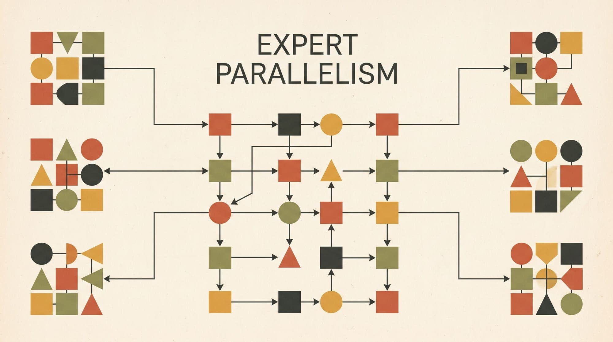
This operational paradigm is known as Expert Parallelism (EP). Rather than slicing individual weight matrices (as in Tensor Parallelism) or sharding layers across time (as in Pipeline Parallelism), Expert Parallelism distributes discrete expert modules across accelerators and utilizes collective All-to-All network primitives to route tokens to their designated expert ranks.

The Distributed MoE Dilemma: Dense vs. Sparse Sharding

In standard Transformer blocks, attention projections and multi-layer perceptrons (MLPs) are identical across all tokens. In an MoE layer, the standard MLP is replaced with $E$ independent expert MLPs and a parameterized gating router:

$y = \sum_{i \in \text{TopK}(G(x), k)} g_i(x) \cdot \text{Expert}_i(x)$

Where $x \in \mathbb{R}^{B \times S \times H}$ represents the hidden representations (with batch size $B$ , sequence length $S$ , and hidden dimension $H$ ), $G(x) \in \mathbb{R}^E$ produces normalized gating logits, and $k \ll E$ defines the active expert count per token.

Applying conventional parallelism to MoE architectures presents severe efficiency limits:

Pure Data Parallelism (DP): Replicates all $E$ experts on every GPU. When $E$ grows to 64, 128, or 256, total model parameters exceed the High Bandwidth Memory (HBM) capacity of a single GPU, rendering pure replication impossible.
Pure Tensor Parallelism (TP): Slices each individual expert weight matrix across $TP$ GPUs. When experts are fine-grained (having smaller intermediate dimensions), the compute intensity per GPU drops significantly. This creates high kernel launch overhead and memory bandwidth underutilization while incurring heavy All-Reduce latency on every expert forward pass.
Pure Pipeline Parallelism (PP): Shards entire MoE layers across pipeline stages, which preserves memory but fails to exploit intra-layer expert concurrency and introduces pipeline bubbles.

Expert Parallelism solves this by assigning different subsets of experts to different GPU workers. Non-MoE components (self-attention, layer normalizations, embeddings) run under standard Data Parallelism, Tensor Parallelism, or Sequence Parallelism, while MoE layers transition into an expert-parallel process group.

The Execution Pipeline: All-to-All Token Dispatch and Combine

Because each GPU hosts only a subset of the total experts, a token processed by GPU $A$ in the self-attention layer may need to be evaluated by an expert hosted on GPU $B$ . This requires a dynamic, two-phase routing cycle during the forward pass:

All-to-All Token Dispatch and Combine Pipeline in Expert Parallelism

1. Router Gating and Softmax Selection

The gating network computes routing probabilities across all $E$ experts for each local token $x_t$ . The router selects the top- $k$ expert indices and normalizes their gating weights:

$g_t = \text{Softmax}(\text{TopK}(W_g x_t, k))$

Each token is replicated $k$ times, pairing each instance with its target expert ID and destination GPU rank.

2. Local Token Permutation

Tokens are physically reordered and binned in GPU memory according to their destination ranks. Instead of sending tokens individually, the local engine groups tokens bound for the same remote GPU into contiguous memory buffers to maximize network packet efficiency.

3. All-to-All Token Dispatch

The cluster executes an All-to-All-v (vectorized All-to-All) collective communication primitive. In this phase:

Every GPU sends its outgoing token buffers to their respective destination GPUs.
Every GPU receives incoming token buffers that target the specific experts hosted locally.

Unlike standard All-to-All, which requires fixed-size transfers between all pairs, All-to-All-v accommodates variable token counts per GPU pair.

4. Local Expert Computation

Once received, tokens are unpacked and routed to their local expert networks. Because multiple tokens from different original GPUs may target the same local expert, the execution engine packs them into a single batched General Matrix Multiply (GEMM) operation:

$h_{\text{out}} = W_2 \cdot \text{SiLU}(W_1 h_{\text{in}} \odot W_3 h_{\text{in}})$

5. All-to-All Token Combine

After local expert MLPs complete their forward projections, the resulting activation vectors must be returned to their originating GPUs. A second All-to-All-v collective communication step transmits the expert output vectors back across the interconnect.

6. Unpermutation and Weighted Reduction

The originating GPU receives the expert outputs, restores them to their original sequence positions, multiplies each output by its corresponding gating weight $g_t$ , and sums the $k$ expert outputs before adding the residual connection.

Backward Pass Symmetry

During backpropagation, the communication pattern is precisely mirrored:

Upstream activation gradients $\frac{\partial \mathcal{L}}{\partial y}$ are dispatched back to the expert GPUs via an All-to-All collective.
Expert GPUs compute local weight gradients $\nabla W_{\text{expert}}$ and input activation gradients $\frac{\partial \mathcal{L}}{\partial x_{\text{expert}}}$ .
Input activation gradients are returned to the originating attention GPUs via a final All-to-All combine collective.

Communication Volume and Hardware Topology

A critical distinction between Expert Parallelism and standard data or tensor parallelism lies in communication volume scaling.

In Data Parallelism and Tensor Parallelism, collective communication (All-Reduce or Reduce-Scatter / All-Gather) depends on the size of the model parameters or activation tensors, remaining constant regardless of batch size. In Expert Parallelism, All-to-All communication volume scales directly with batch size, sequence length, and top- $k$ routing.

The data volume transferred per GPU during a single forward pass All-to-All dispatch is given by:

$\text{Volume}_{\text{dispatch}} = B \times S \times k \times H \times \left(\frac{\text{EP} - 1}{\text{EP}}\right) \times \text{sizeof}(\text{dtype})$

Where $\text{EP}$ is the Expert Parallel size. Across both forward dispatch and combine phases (and doubled again during the backward pass), the total communication volume for an MoE layer is:

$\text{Volume}_{\text{total, layer}} = 4 \times B \times S \times k \times H \times \left(\frac{\text{EP} - 1}{\text{EP}}\right) \times \text{sizeof}(\text{dtype})$

The Cross-Node Bandwidth Barrier

When $\text{EP} \le 8$ , all expert communication occurs within a single server node over high-speed NVLink (offering 900 GB/s to 1.8 TB/s per GPU). At this bandwidth, All-to-All overhead is minimal.

However, when scaling to large MoE clusters with $\text{EP} = 16, 32,$ or $64$ , token dispatch must traverse cross-node networking (InfiniBand or RoCE at 400 Gbps to 800 Gbps, corresponding to 50 to 100 GB/s per GPU). Because inter-node bandwidth is an order of magnitude lower than NVLink, unoptimized cross-node All-to-All becomes the primary execution bottleneck.

Managing Token Imbalance: Capacity Factors vs. Dropless Dispatch

Because routing is dynamic and input-dependent, tokens do not distribute uniformly across experts. Certain "celebrity experts" may receive a disproportionately high share of tokens, while others remain underutilized.

This creates two critical failure modes:

Computational Stragglers: GPUs hosting oversubscribed experts take longer to finish local GEMMs, forcing all other GPUs in the All-to-All group to idle at the barrier.
Memory Spikes and OOM: If token buffers exceed pre-allocated GPU memory, the runtime crashes.

+-------------------------------------------------------------+
|               Router Gating & Token Routing                 |
| Token 1 -> Expert 2 (GPU 0)    Token 3 -> Expert 8 (GPU 1)  |
| Token 2 -> Expert 2 (GPU 0)    Token 4 -> Expert 2 (GPU 0)  |
+-------------------------------------------------------------+
                               |
               [Unbalanced Token Distribution]
                               |
                +--------------+--------------+
                |                             |
                v                             v
     +--------------------+        +--------------------+
     |       GPU 0        |        |       GPU 1        |
     | Expert 2 (3 tokens)|        | Expert 8 (1 token) |
     | Oversubscribed     |        | Underutilized      |
     +--------------------+        +--------------------+

Static Capacity Factors and Token Dropping

Pioneered by GShard and Switch Transformers, static buffer allocation defines an Expert Capacity ( $C_{\text{expert}}$ ):

$C_{\text{expert}} = \text{ceil}\left(\text{Capacity Factor} \times \frac{k \times B \times S}{E}\right)$

The Capacity Factor ( $CF$ ) dictates buffer headroom:

$CF = 1.0$ : Buffers match perfectly balanced load. Any imbalance causes overflow, and dropped tokens bypass the expert layer via residual connections without computation.
$CF = 1.25$ to $1.5$ : Provides 25% to 50% extra buffer headroom to absorb routing spikes, reducing token drop rates at the expense of padding empty slots and consuming extra HBM.

To encourage balanced routing, models typically train with an auxiliary load balancing loss ( $\mathcal{L}_{\text{aux}}$ ):

$\mathcal{L}_{\text{aux}} = \alpha \cdot E \sum_{i=1}^{E} f_i \cdot P_i$

Where $f_i$ is the fraction of tokens dispatched to expert $i$ , $P_i$ is the router probability allocated to expert $i$ , and $\alpha$ is a hyperparameter scaling factor.

Modern Dropless Dynamic Dispatch

While static capacity factors simplify static memory management, dropping tokens during inference degrades model reasoning quality. Modern serving engines (such as DeepSpeed-MoE, Tutel, and Megatron-Core) implement dynamic, dropless dispatch kernels.

Dropless dispatch dynamically resizes communication buffers and utilizes ragged batched GEMMs (e.g., grouped GEMM / cutlass extensions) to process exact token counts per expert without zero-padding or token loss. In DeepSeek-V3, an auxiliary-loss-free load balancing strategy applies dynamically adjusted bias terms to expert routing scores, maintaining hardware balance without distorting the underlying model representations.

Multi-Dimensional Parallelism and Parallel Folding

In large-scale clusters, Expert Parallelism is rarely deployed in isolation. It is composed with Tensor Parallelism (TP), Pipeline Parallelism (PP), Context Parallelism (CP), and Data Parallelism (DP/FSDP).

The Classical $EP \le DP$ Constraint

In early distributed MoE implementations, Expert Parallelism was strictly constrained as a subgroup of Data Parallelism ( $EP \le DP$ ). GPUs sharing the same expert group acted as data-parallel replicas for attention layers while sharding experts for MoE layers.

This coupling creates severe architectural friction:

Attention layers benefit from Tensor Parallelism to distribute large attention heads and sequence lengths.
MoE layers suffer under Tensor Parallelism because sharding already-narrow expert intermediate dimensions results in memory-bandwidth-bound GEMMs with poor GPU utilization.

MoE Parallel Folding

To eliminate these trade-offs, modern distributed frameworks like Megatron-Core MoE introduce Parallel Folding (also known as Heterogeneous Parallelism Mapping).

+-------------------------------------------------------------------------+
|                  Heterogeneous Parallelism Mapping                      |
+-------------------------------------------------------------------------+
| Attention Block:                                                        |
| [GPU 0, GPU 1, GPU 2, GPU 3] -> Tensor Parallel = 4, Context Parallel = 2|
+-------------------------------------------------------------------------+
                                    |
                    [Parallel Folding Re-sharding]
                                    |
+-------------------------------------------------------------------------+
| MoE Block:                                                              |
| [GPU 0] -> Expert 1..8       [GPU 2] -> Expert 17..24                   |
| [GPU 1] -> Expert 9..16      [GPU 3] -> Expert 25..32                   |
| (Tensor Parallel = 1, Expert Parallel = 4, Pure Local GEMMs)            |
+-------------------------------------------------------------------------+

Parallel Folding decouples the process group topologies between attention blocks and MoE blocks:

Attention Layers: Run with higher Tensor Parallelism ( $TP > 1$ ) and Context Parallelism ( $CP > 1$ ) to handle large sequence lengths and multi-head attention state efficiently.
MoE Layers: Automatically collapse $TP \to 1$ and scale $EP$ across the entire available GPU pool. This keeps individual expert computations whole, maximizing GEMM arithmetic intensity on Tensor Cores.

Overlapping All-to-All with Computation

Because cross-node All-to-All communication can stall execution pipelines, modern architectures employ asynchronous dual-stream scheduling. In DeepSeek-V3 and Megatron-Core, token dispatch for MoE layer $l+1$ is initiated asynchronously while GPU Tensor Cores are actively executing the attention projections or shared expert computations of layer $l$ .

By overlapping network packet transmission with dense compute, the communication overhead of Expert Parallelism is largely hidden behind compute execution times.

Distributed Parallelism Strategies Compared

Architectural Implications for Frontier LLMs

Expert Parallelism has become a cornerstone of modern frontier AI architectures. By decoupling parameter capacity from compute throughput, models like DeepSeek-V3, Mixtral 8x22B, and Switch Transformers achieve state-of-the-art reasoning quality at a fraction of the inference and training FLOPS required by equivalent dense models.

However, moving from dense compute to sparse routing shifts the primary engineering challenge from raw arithmetic throughput to interconnect bandwidth and collective communication scheduling. Understanding All-to-All dispatch mechanics, capacity factor dynamics, and parallel folding topologies is essential for training and serving large-scale MoE systems efficiently.

Expert Parallelism in Large Language Models: How All-to-All Token Dispatch, Capacity Factors, and Parallel Folding Scale MoE Architectures

Expert Parallelism in Large Language Models: How All-to-All Token Dispatch, Capacity Factors, and Parallel Folding Scale MoE Architectures

The Distributed MoE Dilemma: Dense vs. Sparse Sharding