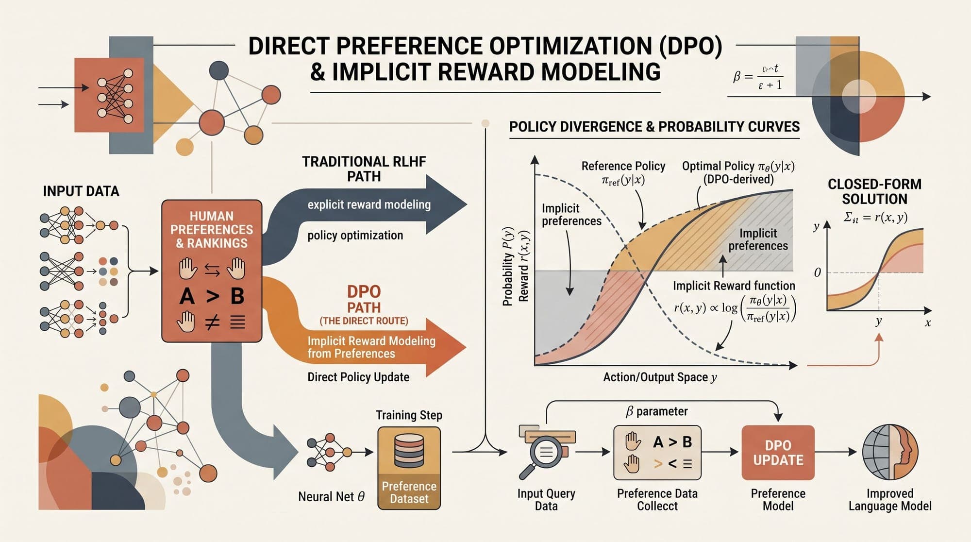
Direct Preference Optimization (DPO): Mathematical Foundations, Implicit Reward Derivation, Closed-Form Bradley-Terry Equivalence, and Reference Policy Regularization

Post-training preference alignment is the central mechanism for transforming pretrained base large language models into instruction-following, steerable, and safe conversational agents. Historically, the dominant paradigm for preference alignment has been Reinforcement Learning from Human Feedback (Christiano et al., 2017; Ouyang et al., 2022), which relies on a multi-stage pipeline: fitting an explicit scalar reward model to human comparison pairs and then optimizing the policy using policy gradient algorithms such as Proximal Policy Optimization (Schulman et al., 2017).

Despite its empirical success, the standard RLHF pipeline introduces substantial systemic complexity. It requires managing four distinct neural networks in GPU memory (actor, critic, reward model, and reference model), generates dynamic rollouts on the fly during training, and suffers from extreme hyperparameter sensitivity and training instability.

To resolve these computational and algorithmic hurdles, Rafailov et al. (2023) introduced Direct Preference Optimization (DPO). DPO proves that the constrained reinforcement learning problem can be solved in closed form. By establishing an exact mathematical equivalence between the optimal policy and the underlying reward function, DPO parameterizes the reward model implicitly through the language model policy itself. This analytical substitution eliminates the need for an explicit reward model, removes the reinforcement learning inner loop, and reduces preference optimization to a stable, closed-form binary cross-entropy loss over static offline preference pairs.

This technical guide provides a rigorous derivation of the mathematical foundations of DPO, analyzes its gradient dynamics and implicit reward mechanics, explores regularization dynamics governed by the temperature parameter $\beta$, compares DPO against alternative alignment paradigms, and provides a standalone production PyTorch implementation.

1. Classical RLHF and the Constrained Optimization Objective

To understand DPO, we must first formalize the constrained optimization objective that underpins standard RLHF.

The Constrained RL Objective

Let $x \sim \mathcal{D}$ denote a prompt sampled from a dataset distribution, and let $y \sim \pi(y \mid x)$ denote a sequence of tokens generated by a parameterized language model policy $\pi_\theta$. In the standard RLHF framework, we seek a policy that maximizes an expected reward $r(x, y)$ while penalizing divergence from a frozen reference policy $\pi_{\text{ref}}(y \mid x)$ (typically the supervised fine-tuned checkpoint). Divergence is measured via the Kullback-Leibler (KL) divergence to prevent the policy from drifting into degenerate output modes or exploiting reward model vulnerabilities (reward hacking).

The mathematical objective is formulated as:

$$\max_{\pi} \mathbb{E}_{x \sim \mathcal{D}} \left[ \mathbb{E}_{y \sim \pi(y \mid x)} \left[ r(x, y) \right] - \beta D_{\text{KL}}\left(\pi(y \mid x) \parallel \pi_{\text{ref}}(y \mid x)\right) \right]$$

where $\beta > 0$ is a scalar hyperparameter that controls the strength of the KL divergence penalty.

The Kullback-Leibler divergence between $\pi(y \mid x)$ and $\pi_{\text{ref}}(y \mid x)$ is defined as:

$$D_{\text{KL}}\left(\pi(y \mid x) \parallel \pi_{\text{ref}}(y \mid x)\right) = \mathbb{E}_{y \sim \pi(y \mid x)} \left[ \log \frac{\pi(y \mid x)}{\pi_{\text{ref}}(y \mid x)} \right]$$

Substituting this definition into the objective yields:

$$\max_{\pi} \mathbb{E}_{x \sim \mathcal{D}, y \sim \pi(y \mid x)} \left[ r(x, y) - \beta \log \frac{\pi(y \mid x)}{\pi_{\text{ref}}(y \mid x)} \right]$$

The Bradley-Terry Preference Model

In classical RLHF, the ground-truth reward function $r(x, y)$ is unobserved. Instead, we observe discrete human or automated preferences over pairs of completions. Given a prompt $x$ and two candidate completions $(y_1, y_2)$, a label $y_w \succ y_l$ indicates that completion $y_w$ (the chosen response) is preferred over completion $y_l$ (the rejected response).

Preferences are assumed to follow the Bradley-Terry-Luce (BTL) model:

$$P(y_1 \succ y_2 \mid x) = \sigma\left(r(x, y_1) - r(x, y_2)\right) = \frac{1}{1 + \exp\left(-(r(x, y_1) - r(x, y_2))\right)}$$

where $\sigma(z) = \frac{1}{1 + e^{-z}}$ is the standard logistic sigmoid function.

Under classical RLHF, a parameterized reward model $r_\phi(x, y)$ is trained via maximum likelihood estimation by minimizing the binary cross-entropy loss over a dataset of static preference pairs $\mathcal{D}_{\text{pref}} = \{(x^{(i)}, y_w^{(i)}, y_l^{(i)})\}_{i=1}^N$:

$$\mathcal{L}_R(\phi) = - \mathbb{E}_{(x, y_w, y_l) \sim \mathcal{D}_{\text{pref}}} \left[ \log \sigma\left(r_\phi(x, y_w) - r_\phi(x, y_l)\right) \right]$$

Once $r_\phi$ is trained and frozen, Proximal Policy Optimization (PPO) optimizes $\pi_\theta$ against $r_\phi(x, y)$ in an online reinforcement learning loop.

2. Mathematical Derivation of the Optimal Policy and Implicit Reward

The breakthrough of Direct Preference Optimization lies in demonstrating that the constrained RL objective possesses an analytical, closed-form solution for any arbitrary reward function $r(x, y)$, and that this relationship can be inverted to express the reward directly in terms of the optimal policy.

Step 1: Deriving the Optimal Policy $\pi^*(y \mid x)$

Consider the per-prompt objective for a fixed prompt $x$:

$$\max_{\pi} \sum_{y} \pi(y \mid x) r(x, y) - \beta \sum_{y} \pi(y \mid x) \log \frac{\pi(y \mid x)}{\pi_{\text{ref}}(y \mid x)}$$

subject to the probability simplex constraint:

$$\sum_{y} \pi(y \mid x) = 1, \quad \forall y: \pi(y \mid x) \ge 0$$

Factoring out $-\beta$, we can rewrite the objective inside the maximization as:

$$\mathcal{J}(\pi) = -\beta \sum_{y} \pi(y \mid x) \left[ \log \frac{\pi(y \mid x)}{\pi_{\text{ref}}(y \mid x)} - \frac{1}{\beta} r(x, y) \right]$$

Using the properties of logarithms, $\frac{1}{\beta} r(x, y) = \log \exp\left(\frac{1}{\beta} r(x, y)\right)$. Thus:

$$\mathcal{J}(\pi) = -\beta \sum_{y} \pi(y \mid x) \left[ \log \left( \frac{\pi(y \mid x)}{\pi_{\text{ref}}(y \mid x) \exp\left(\frac{1}{\beta} r(x, y)\right)} \right) \right]$$

To convert the denominator into a valid, normalized probability distribution over all possible completions $y$, define the partition function $Z(x)$:

$$Z(x) = \sum_{y} \pi_{\text{ref}}(y \mid x) \exp\left(\frac{1}{\beta} r(x, y)\right)$$

Multiplying and dividing the denominator inside the logarithm by $Z(x)$ yields:

$$\mathcal{J}(\pi) = -\beta \sum_{y} \pi(y \mid x) \left[ \log \left( \frac{\pi(y \mid x)}{\frac{1}{Z(x)} \pi_{\text{ref}}(y \mid x) \exp\left(\frac{1}{\beta} r(x, y)\right)} \cdot \frac{1}{Z(x)} \right) \right]$$

$$\mathcal{J}(\pi) = -\beta \sum_{y} \pi(y \mid x) \log \left( \frac{\pi(y \mid x)}{\frac{1}{Z(x)} \pi_{\text{ref}}(y \mid x) \exp\left(\frac{1}{\beta} r(x, y)\right)} \right) + \beta \sum_{y} \pi(y \mid x) \log Z(x)$$

Since $\sum_y \pi(y \mid x) = 1$, the term $\beta \sum_y \pi(y \mid x) \log Z(x)$ simplifies to $\beta \log Z(x)$.

Now, define the normalized distribution $\pi^*(y \mid x)$:

$$\pi^*(y \mid x) = \frac{1}{Z(x)} \pi_{\text{ref}}(y \mid x) \exp\left(\frac{1}{\beta} r(x, y)\right)$$

Substituting $\pi^*(y \mid x)$ back into the objective:

$$\mathcal{J}(\pi) = -\beta D_{\text{KL}}\left(\pi(y \mid x) \parallel \pi^*(y \mid x)\right) + \beta \log Z(x)$$

Because the partition function $Z(x)$ does not depend on the policy $\pi(y \mid x)$, maximizing $\mathcal{J}(\pi)$ is strictly equivalent to minimizing the Kullback-Leibler divergence $D_{\text{KL}}\left(\pi(y \mid x) \parallel \pi^*(y \mid x)\right)$.

Since KL divergence is strictly non-negative ($D_{\text{KL}} \ge 0$) and attains its global minimum of zero if and only if the two distributions are identical everywhere, the unique optimal policy $\pi^*(y \mid x)$ is the Gibbs distribution:

$$\pi^*(y \mid x) = \frac{1}{Z(x)} \pi_{\text{ref}}(y \mid x) \exp\left(\frac{1}{\beta} r(x, y)\right)$$

Step 2: Inverting for the Implicit Reward Function

We now invert this closed-form relation to express the ground-truth reward $r(x, y)$ as a function of the optimal policy $\pi^*$ and the reference policy $\pi_{\text{ref}}$.

Taking the natural logarithm of both sides:

$$\log \pi^*(y \mid x) = \log \pi_{\text{ref}}(y \mid x) + \frac{1}{\beta} r(x, y) - \log Z(x)$$

Rearranging for $r(x, y)$:

$$\frac{1}{\beta} r(x, y) = \log \frac{\pi^*(y \mid x)}{\pi_{\text{ref}}(y \mid x)} + \log Z(x)$$

$$r(x, y) = \beta \log \frac{\pi^*(y \mid x)}{\pi_{\text{ref}}(y \mid x)} + \beta \log Z(x)$$

This derivation reveals that any optimal policy $\pi^*(y \mid x)$ uniquely defines an implicit scalar reward function up to an additive constant $\beta \log Z(x)$ that depends solely on the prompt $x$.

3. Closed-Form Bradley-Terry Substitution and the DPO Loss

In the classical reward modeling objective, preferences depend on the scalar reward difference between two completions $y_w$ and $y_l$ evaluated on the same prompt $x$:

$$P(y_w \succ y_l \mid x) = \sigma\left(r(x, y_w) - r(x, y_l)\right)$$

Substituting our derived expression for $r(x, y)$ into the reward difference:

$$r(x, y_w) - r(x, y_l) = \left( \beta \log \frac{\pi^<em>(y_w \mid x)}{\pi_{\text{ref}}(y_w \mid x)} + \beta \log Z(x) \right) - \left( \beta \log \frac{\pi^</em>(y_l \mid x)}{\pi_{\text{ref}}(y_l \mid x)} + \beta \log Z(x) \right)$$

Crucially, the intractable partition function term $\beta \log Z(x)$ cancels out identically:

$$r(x, y_w) - r(x, y_l) = \beta \log \frac{\pi^<em>(y_w \mid x)}{\pi_{\text{ref}}(y_w \mid x)} - \beta \log \frac{\pi^</em>(y_l \mid x)}{\pi_{\text{ref}}(y_l \mid x)}$$

$$r(x, y_w) - r(x, y_l) = \beta \left( \log \frac{\pi^<em>(y_w \mid x)}{\pi_{\text{ref}}(y_w \mid x)} - \log \frac{\pi^</em>(y_l \mid x)}{\pi_{\text{ref}}(y_l \mid x)} \right)$$

The Direct Preference Optimization Objective

Replacing the theoretical optimal policy $\pi^*$ with our parameterized language model policy $\pi_\theta$, we can express the probability of the preference pair directly under the policy $\pi_\theta$:

$$P_\theta(y_w \succ y_l \mid x) = \sigma\left( \beta \log \frac{\pi_\theta(y_w \mid x)}{\pi_{\text{ref}}(y_w \mid x)} - \beta \log \frac{\pi_\theta(y_l \mid x)}{\pi_{\text{ref}}(y_l \mid x)} \right)$$

Applying maximum likelihood estimation over the offline dataset of pairwise preferences $\mathcal{D}$, we formulate the DPO Loss Function:

$$\mathcal{L}_{\text{DPO}}(\theta; \pi_{\text{ref}}) = - \mathbb{E}_{(x, y_w, y_l) \sim \mathcal{D}} \left[ \log \sigma \left( \beta \log \frac{\pi_\theta(y_w \mid x)}{\pi_{\text{ref}}(y_w \mid x)} - \beta \log \frac{\pi_\theta(y_l \mid x)}{\pi_{\text{ref}}(y_l \mid x)} \right) \right]$$

By defining the implicit reward estimator as:

$$\hat{r}_\theta(x, y) = \beta \log \frac{\pi_\theta(y \mid x)}{\pi_{\text{ref}}(y \mid x)}$$

the DPO loss is written compactly as:

$$\mathcal{L}_{\text{DPO}}(\theta; \pi_{\text{ref}}) = - \mathbb{E}_{(x, y_w, y_l)} \left[ \log \sigma \left( \hat{r}_\theta(x, y_w) - \hat{r}_\theta(x, y_l) \right) \right]$$

4. Gradient Mechanics and Optimization Dynamics

To understand how DPO updates model parameters during training, we compute the analytical gradient of $\mathcal{L}_{\text{DPO}}(\theta)$ with respect to $\theta$.

Let $u = \hat{r}_\theta(x, y_w) - \hat{r}_\theta(x, y_l) = \beta \log \frac{\pi_\theta(y_w \mid x)}{\pi_{\text{ref}}(y_w \mid x)} - \beta \log \frac{\pi_\theta(y_l \mid x)}{\pi_{\text{ref}}(y_l \mid x)}$.

The loss is $\mathcal{L} = -\log \sigma(u)$. The derivative of $-\log \sigma(u)$ with respect to $u$ is:

$$\frac{d}{du} \left[ -\log \sigma(u) \right] = -(1 - \sigma(u)) = -\sigma(-u)$$

Applying the chain rule:

$$\nabla_\theta \mathcal{L}_{\text{DPO}}(\theta) = -\beta \mathbb{E}_{(x, y_w, y_l)} \left[ \sigma\left(\hat{r}_\theta(x, y_l) - \hat{r}_\theta(x, y_w)\right) \left[ \nabla_\theta \log \pi_\theta(y_w \mid x) - \nabla_\theta \log \pi_\theta(y_l \mid x) \right] \right]$$

Deconstruction of the Gradient Components

The gradient vector decomposes into two primary terms:

1. Directional Push-Pull Dynamics:

$$\nabla_\theta \log \pi_\theta(y_w \mid x) - \nabla_\theta \log \pi_\theta(y_l \mid x)$$ This term simultaneously increases the log-likelihood of the preferred sequence $y_w$ (likelihood maximization) while decreasing the log-likelihood of the dispreferred sequence $y_l$ (unlikelihood minimization).

1. Adaptive Error Weighting Factor:

$$w(x, y_w, y_l) = \sigma\left(\hat{r}_\theta(x, y_l) - \hat{r}_\theta(x, y_w)\right) = 1 - \sigma\left(\hat{r}_\theta(x, y_w) - \hat{r}_\theta(x, y_l)\right)$$ This scalar weight measures how incorrectly the current model scores the pair:

• Incorrect ordering ($\hat{r}_\theta(x, y_l) \gg \hat{r}_\theta(x, y_w)$): $w \to 1$. The gradient magnitude is maximized, strongly adjusting the parameters to flip the preference ranking.
• Correct ordering ($\hat{r}_\theta(x, y_w) \gg \hat{r}_\theta(x, y_l)$): $w \to 0$. The gradient vanishes, preventing over-optimization on pairs where the model already exhibits the correct margin.

5. Hyperparameter $\beta$ and Regularization Dynamics

The parameter $\beta$ acts as an inverse temperature that regulates the trade-off between maximizing implicit reward and staying close to the reference model.

Low Beta (e.g., 0.01)                     High Beta (e.g., 0.50)
◄──────────────────────────────────────────────────────────────►
- Weak KL constraint                      - Strong KL constraint
- Rapid policy drift                      - Conservative parameter updates
- High risk of token degeneration         - Slower preference convergence
- Sharp log-ratio separation              - Tight anchoring to SFT base

The Role of $\beta$ in Gradient Scaling and Implicit Margin

From the gradient formula:

• If $\beta$ is set too high ($\beta > 0.5$), the weighting term $\sigma(\beta (\dots))$ saturates slowly, and the policy remains rigidly anchored to $\pi_{\text{ref}}$, resulting in slow learning.
• If $\beta$ is set too low ($\beta < 0.01$), the implicit reward scale $\hat{r}_\theta = \beta \log(\pi_\theta / \pi_{\text{ref}})$ collapses, causing extreme gradient updates that can destroy the model's base linguistic capabilities.

In practical post-training workflows, default values of $\beta \in [0.05, 0.1]$ provide the optimal balance for 7B to 70B parameter models.

Degeneration Pathology: Likelihood Displacement

A known failure mode of naive DPO training is likelihood displacement. Because DPO penalizes $\log \pi_\theta(y_l \mid x)$, the gradient pushes down token probabilities across the entire dispreferred sequence. If $y_w$ and $y_l$ share extensive common prefixes or valid syntactic tokens, gradient updates on $y_l$ can inadvertently depress the probabilities of correct tokens, leading to repetition loops or degraded prose fluency.

This phenomenon motivated the development of length-regularized and bounded variants such as SimPO (Meng et al., 2024) and Identity Preference Optimization (IPO, Azar et al., 2023).

6. Structural Comparison Across Preference Alignment Methods

The table below contrasts DPO with traditional RLHF and downstream non-RL preference algorithms.

| Paradigm | Reference Paper | Active Models in VRAM | Training Type | Optimization Objective | Reward Modeling | | :--- | :--- | :--- | :--- | :--- | :--- | | PPO (RLHF) | Schulman et al., 2017 | 4 (Actor, Critic, Ref, Reward) | Online RL | Clipped Surrogate Policy Gradient | Explicit Scalar Reward | | DPO | Rafailov et al., 2023 | 2 (Actor $\pi_\theta$, Frozen Ref $\pi_{\text{ref}}$) | Offline Supervised | Pairwise Logistic Loss on Log-Ratios | Implicit Reward Parameterization | | IPO | Azar et al., 2023 | 2 (Actor $\pi_\theta$, Frozen Ref $\pi_{\text{ref}}$) | Offline Supervised | Quadratic Penalty on Log-Ratio Margin | Regularized Implicit Reward | | KTO | Ethayarajh et al., 2024 | 2 (Actor $\pi_\theta$, Frozen Ref $\pi_{\text{ref}}$) | Offline Supervised | Unpaired Prospect Theory Utility Loss | Pointwise Reference Utility | | SimPO | Meng et al., 2024 | 1 (Actor $\pi_\theta$ only) | Offline Supervised | Length-Normalized Margin Loss | Reference-Free Implicit Reward | | ORPO | Hong et al., 2024 | 1 (Actor $\pi_\theta$ only) | Offline Supervised | Monolithic SFT + Log Odds Ratio Penalty | Reference-Free Odds Penalty |

7. Standalone PyTorch Implementation

Below is a self-contained PyTorch implementation of the complete Direct Preference Optimization loss, including forward-pass sequence log-probability calculation, implicit reward extraction, and diagnostic metrics tracking.

import torch
import torch.nn as nn
import torch.nn.functional as F
from typing import Tuple, Dict


class DPOLoss(nn.Module):
    """
    Direct Preference Optimization (DPO) Loss Module.
    
    Implements the analytical closed-form loss from Rafailov et al. (NeurIPS 2023):
    L_DPO = - E_{(x, y_w, y_l)} [ log sigma( beta * log(pi(y_w|x)/pi_ref(y_w|x)) 
                                        - beta * log(pi(y_l|x)/pi_ref(y_l|x)) ) ]
    """
    def __init__(self, beta: float = 0.1, label_smoothing: float = 0.0) -> None:
        super().__init__()
        self.beta = beta
        self.label_smoothing = label_smoothing

    def _get_batch_logps(
        self,
        logits: torch.FloatTensor,
        labels: torch.LongTensor,
        average_log_prob: bool = False
    ) -> torch.FloatTensor:
        """
        Extract token-level log probabilities and compute sequence log-likelihood.
        
        Args:
            logits: Predicted logits of shape (batch_size, seq_len, vocab_size)
            labels: Target token IDs of shape (batch_size, seq_len), where -100 indicates masked tokens
            average_log_prob: Whether to normalize by sequence length
            
        Returns:
            Sequence log probabilities of shape (batch_size,)
        """
        assert logits.shape[:-1] == labels.shape

        # Shift logits and labels for autoregressive next-token prediction
        shift_logits = logits[:, :-1, :].contiguous()
        shift_labels = labels[:, 1:].contiguous()

        # Mask for valid completion tokens
        loss_mask = (shift_labels != -100)

        # Replace -100 with 0 temporarily for gather operation
        clean_labels = shift_labels.clone()
        clean_labels[~loss_mask] = 0

        # Compute log-softmax over vocabulary
        log_probs = F.log_softmax(shift_logits, dim=-1)
        per_token_logps = torch.gather(
            log_probs, dim=2, index=clean_labels.unsqueeze(2)
        ).squeeze(2)

        # Zero-out masked prompt/padding tokens
        per_token_logps = per_token_logps * loss_mask

        # Sum log probabilities over the sequence length
        seq_logps = per_token_logps.sum(dim=-1)

        if average_log_prob:
            seq_lengths = loss_mask.sum(dim=-1).clamp(min=1)
            seq_logps = seq_logps / seq_lengths

        return seq_logps

    def forward(
        self,
        policy_chosen_logps: torch.FloatTensor,
        policy_rejected_logps: torch.FloatTensor,
        reference_chosen_logps: torch.FloatTensor,
        reference_rejected_logps: torch.FloatTensor
    ) -> Tuple[torch.FloatTensor, Dict[str, torch.FloatTensor]]:
        """
        Computes the DPO loss, implicit rewards, and diagnostic metrics.
        
        Args:
            policy_chosen_logps: log pi_theta(y_w | x), shape (B,)
            policy_rejected_logps: log pi_theta(y_l | x), shape (B,)
            reference_chosen_logps: log pi_ref(y_w | x), shape (B,)
            reference_rejected_logps: log pi_ref(y_l | x), shape (B,)
            
        Returns:
            loss: Scalar DPO loss
            metrics: Dictionary containing chosen/rejected rewards, reward margin, and accuracy
        """
        # Calculate log-ratio differences: log(pi_theta / pi_ref)
        pi_logratios_chosen = policy_chosen_logps - reference_chosen_logps
        pi_logratios_rejected = policy_rejected_logps - reference_rejected_logps

        # Implicit rewards scaled by beta
        chosen_rewards = self.beta * pi_logratios_chosen
        rejected_rewards = self.beta * pi_logratios_rejected

        # Implicit reward logit margin
        logits = chosen_rewards - rejected_rewards

        # Binary Cross-Entropy with Optional Label Smoothing
        if self.label_smoothing > 0:
            # Conservative target: (1 - eps) * log(sigmoid(logits)) + eps * log(sigmoid(-logits))
            losses = (
                - (1 - self.label_smoothing) * F.logsigmoid(logits)
                - self.label_smoothing * F.logsigmoid(-logits)
            )
        else:
            losses = -F.logsigmoid(logits)

        loss = losses.mean()

        # Compute Diagnostic Metrics
        with torch.no_grad():
            reward_accuracies = (logits > 0).float().mean()
            reward_margin = (chosen_rewards - rejected_rewards).mean()

        metrics = {
            "loss": loss.detach(),
            "chosen_reward": chosen_rewards.mean().detach(),
            "rejected_reward": rejected_rewards.mean().detach(),
            "reward_margin": reward_margin.detach(),
            "accuracy": reward_accuracies.detach(),
        }

        return loss, metrics


if __name__ == "__main__":
    # Test batch execution
    batch_size = 4
    dpo_criterion = DPOLoss(beta=0.1)

    # Simulated sequence log-probabilities
    pol_chosen = torch.tensor([-12.5, -8.2, -15.1, -9.4])
    pol_rejected = torch.tensor([-18.3, -11.0, -14.9, -14.2])
    ref_chosen = torch.tensor([-13.0, -8.5, -15.0, -9.8])
    ref_rejected = torch.tensor([-15.2, -10.1, -13.5, -12.1])

    loss, metrics = dpo_criterion(pol_chosen, pol_rejected, ref_chosen, ref_rejected)

    print("DPO Loss Execution Verification:")
    for k, v in metrics.items():
        print(f"  {k}: {v.item():.4f}")

8. Production Implementation and Memory Economics

Deploying DPO in enterprise training infrastructure requires addressing memory and compute constraints.

Eliminating Reference Model Memory with Parameter-Efficient Fine-Tuning (PEFT)

Under full-parameter fine-tuning, storing both $\pi_\theta$ and $\pi_{\text{ref}}$ doubles GPU VRAM requirements. However, when using Low-Rank Adaptation (LoRA, Hu et al., 2021), the reference model $\pi_{\text{ref}}$ is simply the frozen base model with adapter weights disabled.

┌─────────────────────────────────────────────────────────────┐
│                    Single Base LLM Weights                  │
│                     (Frozen 16-bit / 4-bit)                 │
└──────────────┬──────────────────────────────┬───────────────┘
               │                              │
               ▼ (Adapter Enabled)            ▼ (Adapter Disabled)
     Active Policy π_θ               Reference Policy π_ref
 (Computes gradients via LoRA)     (Zero additional VRAM footprint)

In an optimized training step:

1. Forward Pass 1 (Policy): Enable LoRA adapter $\rightarrow$ compute $\log \pi_\theta(y_w \mid x)$ and $\log \pi_\theta(y_l \mid x)$.
2. Forward Pass 2 (Reference): Disable LoRA adapter with with torch.no_grad(): $\rightarrow$ compute $\log \pi_{\text{ref}}(y_w \mid x)$ and $\log \pi_{\text{ref}}(y_l \mid x)$.
3. Loss & Backward Pass: Compute $\mathcal{L}_{\text{DPO}}$ and backpropagate gradients exclusively into the LoRA parameters.

This technique eliminates the secondary model VRAM allocation entirely, allowing 70B parameter models to undergo DPO training on standard multi-GPU nodes without multi-node sharding.

Summary of Core Principles

1. Analytical Closed Form: DPO derives the exact global optimum of the KL-constrained RLHF objective, proving that an explicit scalar reward model and PPO policy gradient loop are mathematically redundant.
2. Implicit Reward Parameterization: The reward function is analytically parameterized as $r(x, y) = \beta \log \frac{\pi_\theta(y \mid x)}{\pi_{\text{ref}}(y \mid x)} + \beta \log Z(x)$, where the partition function $Z(x)$ cleanly cancels out in pairwise comparisons.
3. Dual Gradient Force: DPO optimizes parameters by simultaneously increasing the likelihood of preferred completions and decreasing the likelihood of rejected completions, weighted dynamically by the model's current ranking error $\sigma(\hat{r}_\theta(y_l) - \hat{r}_\theta(y_w))$.
4. Zero-Overhead Memory Footprint: When paired with LoRA adapter toggling, DPO requires zero additional memory for the reference model, transforming preference alignment into a stable, single-stage supervised training pass.

Sources

• Direct Preference Optimization: Your Language Model is Secretly a Reward Model (Rafailov et al., NeurIPS 2023 / arXiv:2305.18290)
• Deep Reinforcement Learning from Human Preferences (Christiano et al., NeurIPS 2017 / arXiv:1706.03741)
• Training Language Models to Follow Instructions with Human Feedback (Ouyang et al., NeurIPS 2022 / arXiv:2203.02155)
• Proximal Policy Optimization Algorithms (Schulman et al., 2017 / arXiv:1707.06347)
• A General Theoretical Paradigm to Understand Learning from Human Preferences (Azar et al., 2023 / arXiv:2310.12036)
• SimPO: Simple Preference Optimization with a Reference-Free Reward (Meng et al., NeurIPS 2024 / arXiv:2405.14734)
• ORPO: Monolithic Preference Optimization without Reference Model (Hong et al., EMNLP 2024 / arXiv:2403.07691)
• KTO: Model Alignment as Prospect Theoretic Optimization (Ethayarajh et al., ICML 2024 / arXiv:2402.01306)
• LoRA: Low-Rank Adaptation of Large Language Models (Hu et al., ICLR 2022 / arXiv:2106.09685)