
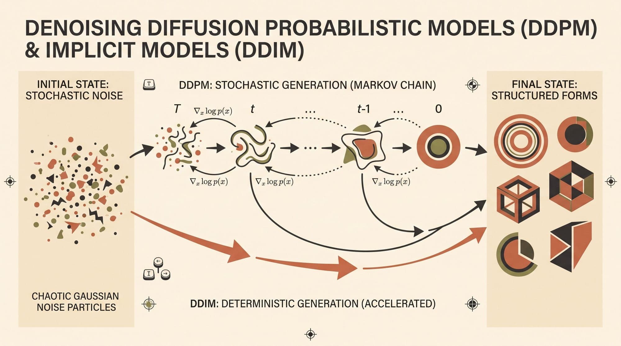
Generative modeling in continuous state spaces underwent a fundamental transformation with the formulation of Denoising Diffusion Probabilistic Models (DDPM) by Ho et al. (2020), building on the non-equilibrium thermodynamics foundations established by Sohl-Dickstein et al. (2015). Prior to diffusion models, deep generative synthesis was dominated by Generative Adversarial Networks (GANs), which suffered from training instability and mode collapse, and Variational Autoencoders (VAEs), which often produced blurry reconstructions due to loose likelihood bounds.
DDPM reframed generation as the reversal of a parameterized discrete-time Markov chain that gradually perturbs data toward an isotropic Gaussian distribution. However, standard DDPM suffered from severe inference latency, requiring up to 1,000 sequential network evaluations to generate a single image. The introduction of Denoising Diffusion Implicit Models (DDIM) by Song et al. (2020) resolved this sampling bottleneck by constructing non-Markovian forward processes that preserve identical marginal distributions while enabling deterministic sampling, exact latent inversion, and a 10x to 50x reduction in sampling steps without retraining the underlying neural network.
This guide provides an end-to-end mathematical derivation of DDPM and DDIM, analyzing the forward Gaussian Markov chain, the variational lower bound (VLB), noise prediction parameterization, variance schedule designs, and the probability flow ordinary differential equation (ODE) formulation.
1. The Forward Gaussian Diffusion Process
The forward diffusion process progressively adds Gaussian noise to a clean data sample x_0 ~ q(x_0) over T discrete timesteps according to a predefined variance schedule beta_1, beta_2, ..., beta_T:
q(x_{1:T} | x_0) = \prod_{t=1}^T q(x_t | x_{t-1})Each individual transition step is modeled as a conditional Gaussian distribution:
q(x_t | x_{t-1}) = N(x_t; \sqrt{1 - beta_t} * x_{t-1}, beta_t * I)where beta_t in (0, 1) represents the variance of the noise injected at step t, and the factor \sqrt{1 - beta_t} scales the mean to maintain bounded variance across transitions.
+-----------+      q(x_1|x_0)      +-----------+      q(x_t|x_{t-1})      +-----------+      q(x_T|x_{t-1})      +-----------+
|    x_0    | -------------------> |    x_1    | -----------------------> |    x_t    | -----------------------> |    x_T    |
| Data Dist |                      |   Noisy   |                          |   Noisy   |                          |  Isotropic|
|           |                      |           |                          |           |                          |  Gaussian |
+-----------+                      +-----------+                          +-----------+                          +-----------+
      ^                                                                         |                                      |
      |                                        q(x_t|x_0)                       |                                      |
      +-------------------------------------------------------------------------+                                      |
      |                                                                                                                |
      |                                        q(x_T|x_0)                                                              |
      +----------------------------------------------------------------------------------------------------------------+
Closed-Form Jump to Arbitrary Timestep t
A foundational property of Gaussian diffusion is that x_t can be sampled directly at any arbitrary timestep t in closed form without iteratively evaluating the intermediate states x_1, ..., x_{t-1}.
Defining alpha_t = 1 - beta_t and the cumulative product \bar{alpha}_t = \prod_{s=1}^t alpha_s, we express x_t recursively using independent standard normal random variables epsilon_1, epsilon_2, ... ~ N(0, I):
x_1 = \sqrt{alpha_1} * x_0 + \sqrt{1 - alpha_1} * epsilon_1x_2 = \sqrt{alpha_2} * x_1 + \sqrt{1 - alpha_2} * epsilon_2
= \sqrt{alpha_2 * alpha_1} * x_0 + \sqrt{alpha_2 * (1 - alpha_1)} * epsilon_1 + \sqrt{1 - alpha_2} * epsilon_2Because the sum of two independent Gaussians N(0, \sigma_a^2 * I) and N(0, \sigma_b^2 * I) is distributed as N(0, (\sigma_a^2 + \sigma_b^2) * I), the variance coefficients combine:
alpha_2 * (1 - alpha_1) + (1 - alpha_2) = alpha_2 - alpha_1 * alpha_2 + 1 - alpha_2 = 1 - alpha_1 * alpha_2 = 1 - \bar{alpha}_2By mathematical induction across t steps:
q(x_t | x_0) = N(x_t; \sqrt{\bar{alpha}_t} * x_0, (1 - \bar{alpha}_t) * I)Equivalently, using the reparameterization trick:
x_t = \sqrt{\bar{alpha}_t} * x_0 + \sqrt{1 - \bar{alpha}_t} * epsilon, where epsilon ~ N(0, I)When the schedule is constructed such that \bar{alpha}_T \approx 0 as T -> \infty, the terminal distribution q(x_T | x_0) converges to standard isotropic Gaussian noise N(0, I), completely destroying the original data distribution q(x_0).
2. Variance Schedules: Linear vs. Cosine
The progression of beta_t determines how quickly information is corrupted during the forward pass.
Linear Schedule
In the original DDPM implementation by Ho et al. (2020), beta_t is linearly interpolated from beta_1 = 10^-4 to beta_T = 0.02 over T = 1,000 steps. While effective for image synthesis on CIFAR-10 and LSUN, the linear schedule destroys visual information too rapidly in early steps (small t) and provides marginal incremental noise at late steps (large t).
Cosine Schedule
To prevent premature signal loss, Nichol and Dhariwal (2021) proposed the cosine variance schedule, defining \bar{alpha}_t directly:
\bar{alpha}_t = f(t) / f(0), where f(t) = \cos((t/T + s) / (1 + s) * \pi / 2)^2where s = 0.008 is a smoothing offset that prevents beta_t from becoming excessively small near t = 0. The corresponding step variance beta_t is derived as:
beta_t = 1 - (\bar{alpha}_t / \bar{alpha}_{t-1}) = 1 - (f(t) / f(t-1))clipped to beta_t <= 0.999 to avoid numerical instabilities at final timesteps.
 Cumulative Signal Retention (\bar{alpha}_t) Comparison
 1.0 |========\
     |         \---\   (Cosine Schedule: Smooth linear degradation)
 0.8 |              \----\
     |                    \----\
 0.6 |                          \----\
     |                               \----\
 0.4 |   \                                 \----\
     |    \                                      \----\
 0.2 |     \--- (Linear Schedule: Fast drop)           \----\
     |         \--------------------------------------------\
 0.0 +-------------------------------------------------------+
     0                     Timestep (t)                    1000
The cosine schedule maintains a roughly linear degradation of image contrast throughout the trajectory, allocating more modeling capacity to intermediate semantic representations.
3. The Reverse Process and Variational Lower Bound
The generative process runs the Markov chain backward from pure Gaussian noise p(x_T) = N(x_T; 0, I) to clean data x_0:
p_\theta(x_{0:T}) = p(x_T) * \prod_{t=1}^T p_\theta(x_{t-1} | x_t)where each reverse transition is parameterized by a neural network with learned mean \mu_\theta(x_t, t) and variance \Sigma_\theta(x_t, t) = \sigma_t^2 * I:
p_\theta(x_{t-1} | x_t) = N(x_{t-1}; \mu_\theta(x_t, t), \Sigma_\theta(x_t, t))Deriving the Variational Bound (L_{VLB})
Training seeks to minimize the negative log-likelihood E[-log p_\theta(x_0)]. Applying Jensen's inequality yields the standard Variational Lower Bound (VLB):
E[-log p_\theta(x_0)] <= E_{q(x_{0:T})} [ log (q(x_{1:T} | x_0) / p_\theta(x_{0:T})) ] = L_{VLB}Expanding the joint probabilities:
L_{VLB} = E_q [ log ( \prod_{t=1}^T q(x_t | x_{t-1}) / (p(x_T) * \prod_{t=1}^T p_\theta(x_{t-1} | x_t)) ) ]Using Bayes' rule to rewrite q(x_t | x_{t-1}) = q(x_{t-1} | x_t, x_0) * q(x_t | x_0) / q(x_{t-1} | x_0), the terms inside the logarithm telescope into three distinct components:
L_{VLB} = E_q [ D_{KL}(q(x_T | x_0) || p(x_T)) + \sum_{t=2}^T D_{KL}(q(x_{t-1} | x_t, x_0) || p_\theta(x_{t-1} | x_t)) - log p_\theta(x_0 | x_1) ]Where each term represents:
- Prior Matching Loss (L_T): The Kullback-Leibler divergence between the final noisy distribution q(x_T | x_0) and standard Gaussian prior p(x_T). Since neither distribution contains learnable parameters, L_T \approx 0 when \bar{alpha}_T \approx 0.
- Denoising Transition Loss (L_{t-1}): Compares the model's reverse transition step p_\theta(x_{t-1} | x_t) against the tractable ground-truth forward posterior q(x_{t-1} | x_t, x_0) conditioned on x_0.
- Reconstruction Loss (L_0): The negative log-likelihood of the final reconstruction step, evaluated using an independent discrete decoder over pixel values.
4. Tractable Forward Posterior q(x_{t-1} | x_t, x_0)
While q(x_{t-1} | x_t) is intractable without knowing the entire data distribution q(x_0), conditioning on x_0 renders the posterior tractable via Bayes' theorem:
q(x_{t-1} | x_t, x_0) = q(x_t | x_{t-1}, x_0) * q(x_{t-1} | x_0) / q(x_t | x_0)
                      = q(x_t | x_{t-1}) * q(x_{t-1} | x_0) / q(x_t | x_0)
Substituting the explicit Gaussian probability density functions:
q(x_{t-1} | x_t, x_0) \propto exp( -0.5 * [ (x_t - \sqrt{alpha_t} * x_{t-1})^2 / beta_t
                                           + (x_{t-1} - \sqrt{\bar{alpha}_{t-1}} * x_0)^2 / (1 - \bar{alpha}_{t-1})
                                           - (x_t - \sqrt{\bar{alpha}_t} * x_0)^2 / (1 - \bar{alpha}_t) ] )
Collecting coefficients of x_{t-1}^2 and x_{t-1} produces a Gaussian distribution N(x_{t-1}; \tilde{\mu}_t(x_t, x_0), \tilde{beta}_t * I):
Posterior Variance (\tilde{beta}_t)
1 / \tilde{beta}_t = (alpha_t / beta_t) + (1 / (1 - \bar{alpha}_{t-1}))
                   = (alpha_t * (1 - \bar{alpha}_{t-1}) + beta_t) / (beta_t * (1 - \bar{alpha}_{t-1}))
                   = (1 - \bar{alpha}_t) / (beta_t * (1 - \bar{alpha}_{t-1}))

\tilde{beta}_t = ((1 - \bar{alpha}_{t-1}) / (1 - \bar{alpha}_t)) * beta_t
Posterior Mean (\tilde{\mu}_t)
\tilde{\mu}_t(x_t, x_0) = [ (\sqrt{alpha_t} / beta_t) * x_t + (\sqrt{\bar{alpha}_{t-1}} / (1 - \bar{alpha}_{t-1})) * x_0 ] * \tilde{beta}_t
                        = (\sqrt{\bar{alpha}_{t-1}} * beta_t / (1 - \bar{alpha}_t)) * x_0
                          + (\sqrt{alpha_t} * (1 - \bar{alpha}_{t-1}) / (1 - \bar{alpha}_t)) * x_t
5. Parameterization and the Simplified Objective
Because q(x_{t-1} | x_t, x_0) and p_\theta(x_{t-1} | x_t) are both multivariate Gaussians with isotropic covariances, their KL divergence at step t has an exact analytical form:
L_{t-1} = E_q [ (1 / (2 * \sigma_t^2)) * || \tilde{\mu}_t(x_t, x_0) - \mu_\theta(x_t, t) ||^2 ] + Cwhere \sigma_t^2 is fixed to either beta_t or \tilde{beta}_t.
Noise Prediction Parameterization
Substituting x_0 = (x_t - \sqrt{1 - \bar{alpha}_t} * epsilon) / \sqrt{\bar{alpha}_t} into the analytical posterior mean \tilde{\mu}_t(x_t, x_0):
\tilde{\mu}_t(x_t, epsilon) = (\sqrt{\bar{alpha}_{t-1}} * beta_t / (1 - \bar{alpha}_t)) * [ (x_t - \sqrt{1 - \bar{alpha}_t} * epsilon) / \sqrt{\bar{alpha}_t} ]
                              + (\sqrt{alpha_t} * (1 - \bar{alpha}_{t-1}) / (1 - \bar{alpha}_t)) * x_t
                            = (1 / \sqrt{alpha_t}) * [ x_t - (beta_t / \sqrt{1 - \bar{alpha}_t}) * epsilon ]
This identity demonstrates that predicting the posterior mean \tilde{\mu}_t is equivalent to training a neural network \epsilon_\theta(x_t, t) to predict the injected Gaussian noise vector epsilon. Setting the model mean to:
\mu_\theta(x_t, t) = (1 / \sqrt{alpha_t}) * [ x_t - (beta_t / \sqrt{1 - \bar{alpha}_t}) * \epsilon_\theta(x_t, t) ]transforms the loss term into:
L_{t-1} = E_{x_0, epsilon} [ (beta_t^2 / (2 * \sigma_t^2 * alpha_t * (1 - \bar{alpha}_t))) * || epsilon - \epsilon_\theta(\sqrt{\bar{alpha}_t} * x_0 + \sqrt{1 - \bar{alpha}_t} * epsilon, t) ||^2 ]The Simplified Loss Function (L_{simple})
Ho et al. (2020) discovered empirically that discarding the scalar weighting prefactor dramatically improves sample visual fidelity:
L_{simple}(\theta) = E_{t ~ U(1, T), x_0, epsilon ~ N(0, I)} [ || epsilon - \epsilon_\theta(\sqrt{\bar{alpha}_t} * x_0 + \sqrt{1 - \bar{alpha}_t} * epsilon, t) ||^2 ]+----------------------------------------------------------------------------------------------------+
| DDPM Training Algorithm |
+----------------------------------------------------------------------------------------------------+
| 1: repeat |
| 2: x_0 ~ q(x_0) // Sample batch of real clean data |
| 3: t ~ Uniform({1, ..., T}) // Sample random timesteps |
| 4: epsilon ~ N(0, I) // Sample Gaussian noise |
| 5: Take gradient descent step on: |
| Grad_theta || epsilon - epsilon_theta( sqrt(alpha_bar_t)*x_0 + |
| sqrt(1 - alpha_bar_t)*epsilon, t ) ||^2 |
| 6: until converged |
+----------------------------------------------------------------------------------------------------+Connection to Denoising Score Matching and Tweedie's Formula
By Tweedie's formula for Gaussian variables, the posterior expectation of x_0 given x_t satisfies:
E[x_0 | x_t] = (x_t + (1 - \bar{alpha}_t) * \nabla_{x_t} log q(x_t)) / \sqrt{\bar{alpha}_t}Comparing this with the reparameterization x_0 = (x_t - \sqrt{1 - \bar{alpha}_t} * epsilon) / \sqrt{\bar{alpha}_t} establishes the direct relationship between the noise prediction model \epsilon_\theta(x_t, t) and the Stein score function \nabla_{x_t} log q(x_t):
\nabla_{x_t} log q(x_t) = - \epsilon_\theta(x_t, t) / \sqrt{1 - \bar{alpha}_t}Training a DDPM network via L_{simple} is mathematically equivalent to multi-scale denoising score matching across varying noise levels \sigma_t = \sqrt{1 - \bar{alpha}_t}.
6. The DDPM Sampling Bottleneck
To sample from a trained DDPM model, one begins with standard Gaussian noise x_T ~ N(0, I) and iteratively steps backward using the reverse Markov chain:
x_{t-1} = (1 / \sqrt{alpha_t}) * [ x_t - (beta_t / \sqrt{1 - \bar{alpha}_t}) * \epsilon_\theta(x_t, t) ] + \sigma_t * zwhere z ~ N(0, I) for t > 1 and z = 0 for t = 1.
+----------------------------------------------------------------------------------------------------+
|                                     DDPM Sampling Algorithm                                        |
+----------------------------------------------------------------------------------------------------+
| 1: x_T ~ N(0, I)                                                                                   |
| 2: for t = T, ..., 1 do                                                                            |
| 3:     z ~ N(0, I) if t > 1, else z = 0                                                            |
| 4:     x_{t-1} = (1 / sqrt(alpha_t)) * (x_t - (beta_t / sqrt(1 - alpha_bar_t)) *                   |
|                  epsilon_theta(x_t, t)) + sigma_t * z                                              |
| 5: end for                                                                                         |
| 6: return x_0                                                                                      |
+----------------------------------------------------------------------------------------------------+
Because each step depends strictly on x_t from the immediately preceding step, generation requires T = 1,000 sequential evaluations of a multi-billion parameter U-Net or Diffusion Transformer (DiT) backbone. This creates an extreme throughput bottleneck in production deployment.
7. Denoising Diffusion Implicit Models (DDIM)
To eliminate the sequential 1,000-step sampling constraint, Song et al. (2020) developed Denoising Diffusion Implicit Models (DDIM). The central insight of DDIM is that the training objective L_{simple} depends solely on the marginal distributions q(x_t | x_0), not on the specific joint Markovian transitions q(x_{1:T} | x_0).

Non-Markovian Forward Process Family
DDIM defines a non-Markovian forward distribution family q_\sigma(x_{1:T} | x_0) conditioned on x_0 that matches the exact Gaussian marginals q_\sigma(x_t | x_0) = N(x_t; \sqrt{\bar{alpha}_t} * x_0, (1 - \bar{alpha}_t) * I):
q_\sigma(x_{1:T} | x_0) = q_\sigma(x_T | x_0) * \prod_{t=2}^T q_\sigma(x_{t-1} | x_t, x_0)The conditional transitions are parameterized by a scalar variance hyperparameter \sigma_t >= 0:
q_\sigma(x_{t-1} | x_t, x_0) = N(x_{t-1}; \sqrt{\bar{alpha}_{t-1}} * x_0 + \sqrt{1 - \bar{alpha}_{t-1} - \sigma_t^2} * ((x_t - \sqrt{\bar{alpha}_t} * x_0) / \sqrt{1 - \bar{alpha}_t}), \sigma_t^2 * I)Generalized Reverse Sampling Trajectory
Given the noise prediction network \epsilon_\theta(x_t, t), the predicted clean sample at step t is:
\hat{x}_0(x_t) = (x_t - \sqrt{1 - \bar{alpha}_t} * \epsilon_\theta(x_t, t)) / \sqrt{\bar{alpha}_t}The generalized reverse step from timestep t to t-1 becomes:
x_{t-1} = \sqrt{\bar{alpha}_{t-1}} * \hat{x}_0(x_t)                       // Predicted x_0 component
          + \sqrt{1 - \bar{alpha}_{t-1} - \sigma_t^2} * \epsilon_\theta(x_t, t)  // Direction pointing to x_t
          + \sigma_t * \epsilon_t                                         // Random noise
where \epsilon_t ~ N(0, I).
Controlling Stochasticity via \sigma_t
The variance \sigma_t controls the degree of randomness in the reverse trajectory:
- Standard DDPM (\sigma_t = \tilde{beta}_t^{1/2}): Setting \sigma_t = \sqrt{(1 - \bar{alpha}_{t-1}) / (1 - \bar{alpha}_t)} * \sqrt{1 - (\bar{alpha}_t / \bar{alpha}_{t-1})} recovers the standard stochastic DDPM Markov chain.
- Deterministic DDIM (\sigma_t = 0): Setting \sigma_t = 0 collapses the random noise term to zero, yielding a fully deterministic trajectory:
x_{t-1} = \sqrt{\bar{alpha}_{t-1}} * [ (x_t - \sqrt{1 - \bar{alpha}_t} * \epsilon_\theta(x_t, t)) / \sqrt{\bar{alpha}_t} ]
          + \sqrt{1 - \bar{alpha}_{t-1}} * \epsilon_\theta(x_t, t)
+----------------------------------------------------------------------------------------------------+
| DDIM Strided Sampling Algorithm |
+----------------------------------------------------------------------------------------------------+
| Input: Sub-sequence of timesteps tau = [tau_1, tau_2, ..., tau_S], where tau_S = T |
| 1: x_{tau_S} ~ N(0, I) |
| 2: for i = S, ..., 1 do |
| 3: t = tau_i, t_prev = tau_{i-1} (with tau_0 = 0, alpha_bar_0 = 1) |
| 4: x_hat_0 = (x_t - sqrt(1 - alpha_bar_t) * epsilon_theta(x_t, t)) / sqrt(alpha_bar_t) |
| 5: dir_xt = sqrt(1 - alpha_bar_{t_prev} - sigma_t^2) * epsilon_theta(x_t, t) |
| 6: noise = sigma_t * epsilon if sigma_t > 0 else 0 |
| 7: x_{t_prev} = sqrt(alpha_bar_{t_prev}) * x_hat_0 + dir_xt + noise |
| 8: end for |
| 9: return x_0 |
+----------------------------------------------------------------------------------------------------+8. Properties of Deterministic DDIM
Setting \sigma_t = 0 unlocks critical capabilities that are impossible in standard stochastic DDPM:
1. Accelerated Sub-Sequence Sampling (10x-50x Speedup)
Because DDIM is not restricted to step-by-step Markovian transitions (t -> t-1), one can select an arbitrary sub-sequence of timesteps \tau = [\tau_1, \tau_2, ..., \tau_S] \subset [1, ..., T] with length S \ll T (e.g. S = 20 or S = 50 steps instead of 1,000). High-quality samples are generated with 10x to 50x fewer function evaluations without retraining \epsilon_\theta.
2. Probability Flow ODE Discretization
As the step size approaches zero in continuous time, the deterministic DDIM update rule corresponds to Euler discretization of the neural Ordinary Differential Equation (ODE):
dx(t) = [ f(x, t) - 0.5 * g(t)^2 * \nabla_x log p_t(x) ] dt
      = [ -0.5 * beta(t) * x(t) + 0.5 * (beta(t) / \sqrt{1 - \bar{alpha}(t)}) * \epsilon_\theta(x(t), t) ] dt
This establishes the direct bridge between discrete DDPM and the continuous-time score-based ODE formulations of Song et al. (2020).
3. Exact Latent Inversion and Semantic Editing
Because the ODE trajectory is deterministic and bidirectional, any real image x_0 can be inverted back into its unique latent noise representation x_T by running the DDIM steps forward in time:
x_{\tau_{i+1}} = \sqrt{\bar{alpha}_{\tau_{i+1}}} * [ (x_{\tau_i} - \sqrt{1 - \bar{alpha}_{\tau_i}} * \epsilon_\theta(x_{\tau_i}, \tau_i)) / \sqrt{\bar{alpha}_{\tau_i}} ]
                + \sqrt{1 - \bar{alpha}_{\tau_{i+1}}} * \epsilon_\theta(x_{\tau_i}, \tau_i)
This latent inversion enables semantic latent space interpolation, image editing, and inpainting without distorting unmasked regions.
9. Architectural Comparison: DDPM vs. DDIM vs. Modern Paradigms
+--------------------+-------------------------+-------------------------+-------------------------+-------------------------+
| Feature            | DDPM (Ho et al., 2020)  | DDIM (Song et al., 2020)| Score SDE (Song, 2020)  | Flow Matching (Lipman)  |
+--------------------+-------------------------+-------------------------+-------------------------+-------------------------+
| Forward Model      | Discrete Markov chain   | Non-Markovian marginals | Continuous SDE          | Continuous vector field |
| Reverse Dynamics   | Stochastic Markov steps | Deterministic ODE / SDE | Reverse SDE / Flow ODE  | Straight-line ODE       |
| Sampling Steps     | 1,000 steps             | 20 to 50 steps          | 20 to 100 steps         | 10 to 30 steps          |
| Latent Inversion   | Impossible (drift)      | Exact (when sigma=0)    | Exact (via ODE flow)    | Exact (via velocity ODE)|
| Retraining Needed  | Baseline                | None (reuses DDPM)      | None (score equivalent) | Yes (vector fields)     |
| Trajectory Type    | Brownian random walk    | Curvilinear ODE flow    | Curved continuous ODE   | Straight transport line |
+--------------------+-------------------------+-------------------------+-------------------------+-------------------------+
Sources
- Denoising Diffusion Probabilistic Models (Ho et al., NeurIPS 2020)
- Denoising Diffusion Implicit Models (Song et al., ICLR 2021)
- Deep Unsupervised Learning using Nonequilibrium Thermodynamics (Sohl-Dickstein et al., ICML 2015)
- Improved Denoising Diffusion Probabilistic Models (Nichol & Dhariwal, ICML 2021)
- Score-Based Generative Modeling through Stochastic Differential Equations (Song et al., ICLR 2021)
- Flow Matching for Generative Modeling (Lipman et al., ICLR 2023)



