Contrastive Preference Optimization (CPO): Mathematical Foundations, Direct Likelihood Regularization, Out-of-Distribution Error Bounds, and Non-Degenerate Policy Alignment

Supervised fine-tuning (SFT) and preference alignment represent the standard two-stage training paradigm for post-training large language models. While SFT establishes foundational task adherence by minimizing cross-entropy loss against target references, it suffers from two structural limitations: it cannot surpass the quality ceiling of its training demonstrations, and it lacks an explicit mechanism to penalize near-correct outputs that contain subtle hallucinations or omissions.

Direct Preference Optimization (Rafailov et al., 2023) addressed these limitations by directly optimizing policy probabilities on paired preference data without training an explicit reward model. However, standard DPO introduces two major operational bottlenecks: it requires maintaining an active reference policy in GPU memory (doubling memory overhead and forward pass compute), and it exhibits a vulnerability termed "likelihood displacement," where the model satisfies the pairwise preference margin by decreasing the probability of both outputs rather than actively boosting the preferred sequence.

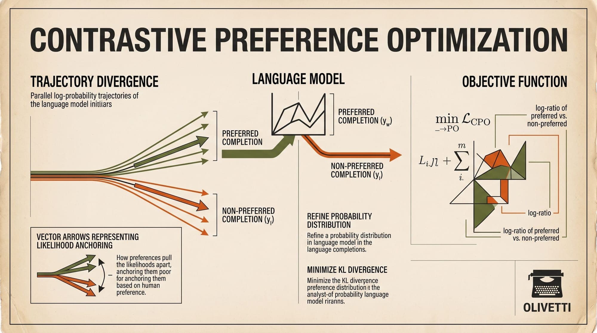
To resolve these challenges, Xu et al. (ICML 2024) introduced Contrastive Preference Optimization (CPO). CPO mathematically reformulates preference optimization by deriving a reference-free upper bound on ideal preference loss and augmenting it with an exact behavior cloning (BC) regularizer. This architecture eliminates the need for an explicit reference model while guaranteeing that the absolute likelihood of high-quality generations remains strictly anchored during alignment.

1. The Limitations of SFT and the DPO Likelihood Displacement Problem

Supervised Fine-Tuning and the Quality Ceiling

In standard supervised fine-tuning over a dataset $\mathcal{D}_{\text{SFT}} = \{(x^{(i)}, y^{(i)})\}_{i=1}^N$ , the model parameters $\theta$ are optimized via empirical risk minimization of the negative log-likelihood (NLL):

$\mathcal{L}_{\text{NLL}}(\theta) = -\mathbb{E}_{(x, y) \sim \mathcal{D}_{\text{SFT}}} \left[ \log \pi_\theta(y|x) \right] = -\mathbb{E}_{(x, y) \sim \mathcal{D}_{\text{SFT}}} \left[ \sum_{t=1}^{|y|} \log \pi_\theta(y_t | x, y_{<t}) \right]$

This objective forces the policy $\pi_\theta$ to match the empirical data distribution $P_{\text{data}}(y|x)$ . In precision-critical domains such as machine translation, formal mathematics, and code synthesis, human-generated references frequently contain subtle noise, non-standard phrasing, or omissions. Research by Freitag et al. (2023) and Xu et al. (2023) demonstrated that strong generative models regularly produce candidate outputs with higher semantic fidelity than human gold references.

Because cross-entropy treats every target token in the dataset as ground truth, SFT cannot penalize outputs that are grammatically coherent but factually incomplete, nor can it exceed the average quality of the demonstration set.

Likelihood Displacement in Direct Preference Optimization

DPO derives a closed-form substitution for the Bradley-Terry reward model:

$r(x, y) = \beta \log \frac{\pi_\theta(y|x)}{\pi_{\text{ref}}(y|x)}$

Under a dataset of pairwise preferences $\mathcal{D}_{\text{pref}} = \{(x^{(i)}, y_w^{(i)}, y_l^{(i)})\}_{i=1}^N$ , where $y_w$ denotes the preferred completion and $y_l$ denotes the dispreferred completion, the standard DPO objective is:

$\mathcal{L}_{\text{DPO}}(\theta; \pi_{\text{ref}}) = -\mathbb{E}_{(x, y_w, y_l) \sim \mathcal{D}_{\text{pref}}} \left[ \log \sigma \left( \beta \log \frac{\pi_\theta(y_w|x)}{\pi_{\text{ref}}(y_w|x)} - \beta \log \frac{\pi_\theta(y_l|x)}{\pi_{\text{ref}}(y_l|x)} \right) \right]$

Let $\Delta r(x, y_w, y_l) = \beta \left( \log \frac{\pi_\theta(y_w|x)}{\pi_{\text{ref}}(y_w|x)} - \log \frac{\pi_\theta(y_l|x)}{\pi_{\text{ref}}(y_l|x)} \right)$. The loss is minimized when $\Delta r \to \infty$ .

However, inspecting the argument of the sigmoid function reveals a mathematical vulnerability:

$\Delta r = \beta \left( \log \pi_\theta(y_w|x) - \log \pi_\theta(y_l|x) \right) - \beta \left( \log \pi_{\text{ref}}(y_w|x) - \log \pi_{\text{ref}}(y_l|x) \right)$

The optimization objective only constrains the relative difference between the log-ratios. If the optimizer encounters a trajectory where $\log \pi_\theta(y_l|x)$ decreases by $10$ units while $\log \pi_\theta(y_w|x)$ simultaneously decreases by $4$ units, the net margin increases by $+6$ units. Consequently, $\mathcal{L}_{\text{DPO}}$ decreases significantly even though the model is actively assigning lower probability to the correct sequence $y_w$ .

In unstructured dialogue, this likelihood displacement often manifests as subtle stylistic shifts. In structured tasks, it leads to severe out-of-distribution hallucinations, repetition loops, and syntax degeneration because the policy drifts away from the valid generation manifold.

2. Mathematical Derivation of the CPO Objective

Contrastive Preference Optimization resolves likelihood displacement by redesigning the objective around two mathematical pillars: a uniform reference upper bound and behavior cloning regularization.

Theorem 1: Uniform Reference Policy as an Upper Bound

Let $\pi_w(y|x)$ denote an ideal oracle policy that perfectly reflects the ground-truth distribution of optimal responses, such that $\pi_w(y_w|x) = 1$ and $0 \le \pi_w(y_l|x) \le 1$ for all $(x, y_w, y_l) \in \mathcal{D}_{\text{pref}}$ .

Substituting $\pi_w$ into the DPO loss yields:

$\mathcal{L}(\pi_\theta; \pi_w) = -\mathbb{E}_{(x, y_w, y_l) \sim \mathcal{D}_{\text{pref}}} \left[ \log \sigma \left( \beta \log \frac{\pi_\theta(y_w|x)}{\pi_w(y_w|x)} - \beta \log \frac{\pi_\theta(y_l|x)}{\pi_w(y_l|x)} \right) \right]$

Since $\log \pi_w(y_w|x) = \log(1) = 0$ , the expression simplifies to:

$\mathcal{L}(\pi_\theta; \pi_w) = -\mathbb{E}_{(x, y_w, y_l) \sim \mathcal{D}_{\text{pref}}} \left[ \log \sigma \left( \beta \log \pi_\theta(y_w|x) - \beta \log \pi_\theta(y_l|x) + \beta \log \pi_w(y_l|x) \right) \right]$

Expanding the logistic sigmoid $\sigma(z) = \frac{1}{1 + e^{-z}}$ :

$\mathcal{L}(\pi_\theta; \pi_w) = -\mathbb{E} \left[ \log \left( \frac{1}{1 + e^{-\beta \log \pi_\theta(y_w|x) + \beta \log \pi_\theta(y_l|x) - \beta \log \pi_w(y_l|x)}} \right) \right]$

$\mathcal{L}(\pi_\theta; \pi_w) = -\mathbb{E} \left[ \log \left( \frac{1}{1 + \frac{\pi_\theta(y_l|x)^\beta}{\pi_\theta(y_w|x)^\beta \cdot \pi_w(y_l|x)^\beta}} \right) \right]$

$\mathcal{L}(\pi_\theta; \pi_w) = -\mathbb{E} \left[ \log \left( \frac{\pi_\theta(y_w|x)^\beta \cdot \pi_w(y_l|x)^\beta}{\pi_\theta(y_w|x)^\beta \cdot \pi_w(y_l|x)^\beta + \pi_\theta(y_l|x)^\beta} \right) \right]$

$\mathcal{L}(\pi_\theta; \pi_w) = -\mathbb{E} \left[ \log \pi_\theta(y_w|x)^\beta + \log \pi_w(y_l|x)^\beta - \log \left( \pi_\theta(y_w|x)^\beta \cdot \pi_w(y_l|x)^\beta + \pi_\theta(y_l|x)^\beta \right) \right]$

Because $\pi_w$ is fixed and independent of the policy parameters $\theta$ , the term $\mathbb{E}[\log \pi_w(y_l|x)^\beta]$ acts as a constant offset $C$ :

$\mathcal{L}'(\pi_\theta; \pi_w) = \mathcal{L}(\pi_\theta; \pi_w) + C = -\mathbb{E} \left[ \log \pi_\theta(y_w|x)^\beta - \log \left( \pi_\theta(y_w|x)^\beta \cdot \pi_w(y_l|x)^\beta + \pi_\theta(y_l|x)^\beta \right) \right]$

where $C = \mathbb{E}_{(x, y_l) \sim \mathcal{D}_{\text{pref}}} [\beta \log \pi_w(y_l|x)]$.

Because $0 \le \pi_w(y_l|x) \le 1$ , we have $\pi_\theta(y_w|x)^\beta \cdot \pi_w(y_l|x)^\beta \le \pi_\theta(y_w|x)^\beta \cdot 1$. Applying this inequality directly:

$\mathcal{L}'(\pi_\theta; \pi_w) \le -\mathbb{E}_{(x, y_w, y_l) \sim \mathcal{D}_{\text{pref}}} \left[ \log \pi_\theta(y_w|x)^\beta - \log \left( \pi_\theta(y_w|x)^\beta + \pi_\theta(y_l|x)^\beta \right) \right]$

Reversing the algebraic expansion:

$-\mathbb{E} \left[ \log \left( \frac{\pi_\theta(y_w|x)^\beta}{\pi_\theta(y_w|x)^\beta + \pi_\theta(y_l|x)^\beta} \right) \right] = -\mathbb{E} \left[ \log \sigma \left( \beta \log \pi_\theta(y_w|x) - \beta \log \pi_\theta(y_l|x) \right) \right]$

Defining $\mathcal{L}(\pi_\theta; U)$ as the reference-free preference loss under a uniform prior $U$ :

$\mathcal{L}_{\text{prefer}}(\theta) = \mathcal{L}(\pi_\theta; U) = -\mathbb{E}_{(x, y_w, y_l) \sim \mathcal{D}_{\text{pref}}} \left[ \log \sigma \left( \beta \log \pi_\theta(y_w|x) - \beta \log \pi_\theta(y_l|x) \right) \right]$

Thus, minimizing $\mathcal{L}_{\text{prefer}}(\theta)$ directly minimizes an upper bound on the ideal preference loss $\mathcal{L}(\pi_\theta; \pi_w) + C$ . This eliminates the requirement to store or evaluate a separate reference model $\pi_{\text{ref}}$ during training.

3. Behavior Cloning Regularization via Constrained KL Duality

Minimizing $\mathcal{L}_{\text{prefer}}(\theta)$ alone still permits relative margin maximization at the expense of absolute probability density. To ensure that $\pi_\theta$ remains strictly bound to the target distribution, CPO introduces a constrained optimization problem:

$\min_\theta \mathcal{L}(\pi_\theta; U) \quad \text{subject to} \quad \mathbb{E}_{(x, y_w) \sim \mathcal{D}_{\text{pref}}} \left[ \mathbb{KL} \left( \pi_w(y_w|x) \,\|\, \pi_\theta(y_w|x) \right) \right] \le \epsilon$

Using Lagrangian duality, this constrained optimization translates to:

$\min_\theta \mathcal{L}(\pi_\theta; U) + \alpha \, \mathbb{E}_{(x, y_w) \sim \mathcal{D}_{\text{pref}}} \left[ \mathbb{KL} \left( \pi_w(y_w|x) \,\|\, \pi_\theta(y_w|x) \right) \right]$

Expanding the Kullback-Leibler divergence over the preferred data distribution:

$\mathbb{KL}\left(\pi_w(y_w|x) \,\|\, \pi_\theta(y_w|x)\right) = \sum_{y \in \mathcal{Y}} \pi_w(y|x) \log \frac{\pi_w(y|x)}{\pi_\theta(y|x)}$

$= \mathbb{E}_{(x, y_w) \sim \mathcal{D}} \left[ \pi_w(y_w|x) \log \pi_w(y_w|x) - \pi_w(y_w|x) \log \pi_\theta(y_w|x) \right]$

Under the ideal oracle distribution where $\pi_w(y_w|x) = 1$ :

$\mathbb{KL}\left(\pi_w(y_w|x) \,\|\, \pi_\theta(y_w|x)\right) = 1 \cdot \log(1) - 1 \cdot \log \pi_\theta(y_w|x) = -\log \pi_\theta(y_w|x)$

Substituting this result directly into the Lagrangian objective produces the final Contrastive Preference Optimization (CPO) loss:

$\mathcal{L}_{\text{CPO}}(\theta) = \underbrace{-\mathbb{E}_{(x, y_w, y_l) \sim \mathcal{D}_{\text{pref}}} \left[ \log \sigma \left( \beta \log \pi_\theta(y_w|x) - \beta \log \pi_\theta(y_l|x) \right) \right]}_{\mathcal{L}_{\text{prefer}}(\theta)} + \alpha \underbrace{\left( -\mathbb{E}_{(x, y_w) \sim \mathcal{D}_{\text{pref}}} \left[ \log \pi_\theta(y_w|x) \right] \right)}_{\mathcal{L}_{\text{NLL}}(\theta)}$

where $\beta > 0$ controls the sensitivity of the contrastive preference boundary and $\alpha > 0$ represents the weighting coefficient for the behavior cloning regularizer (typically set to $\alpha = 1.0$ ).

4. Gradient Flow and Non-Degenerate Policy Updates

To understand why CPO mathematically guarantees non-vanishing probabilities for preferred completions, consider the analytical gradient of $\mathcal{L}_{\text{CPO}}(\theta)$ with respect to the network weights $\theta$ .

Contrastive Preference Optimization Gradient Flow and Likelihood Anchoring

Let $h_\theta(x, y_w, y_l) = \beta \log \pi_\theta(y_w|x) - \beta \log \pi_\theta(y_l|x)$. The derivative of the sigmoid log-loss $\log \sigma(z)$ with respect to $z$ is:

$\frac{\partial \log \sigma(z)}{\partial z} = 1 - \sigma(z) = \sigma(-z)$

Differentiating $\mathcal{L}_{\text{prefer}}(\theta)$ :

$\nabla_\theta \mathcal{L}_{\text{prefer}}(\theta) = -\mathbb{E} \left[ \sigma(-h_\theta) \cdot \beta \left( \nabla_\theta \log \pi_\theta(y_w|x) - \nabla_\theta \log \pi_\theta(y_l|x) \right) \right]$

Differentiating the behavior cloning term $\mathcal{L}_{\text{NLL}}(\theta)$ :

$\nabla_\theta \mathcal{L}_{\text{NLL}}(\theta) = -\mathbb{E} \left[ \nabla_\theta \log \pi_\theta(y_w|x) \right]$

Combining the two components yields the complete CPO gradient:

$\nabla_\theta \mathcal{L}_{\text{CPO}}(\theta) = -\mathbb{E} \left[ \underbrace{\left( \beta \sigma(-h_\theta) + \alpha \right)}_{\text{Positive Anchor Weight}} \nabla_\theta \log \pi_\theta(y_w|x) - \underbrace{\beta \sigma(-h_\theta)}_{\text{Negative Penalty Weight}} \nabla_\theta \log \pi_\theta(y_l|x) \right]$

Analytical Properties of the CPO Gradient

Guaranteed Positive Gradient on Winning Completions: In standard DPO, the gradient coefficient on $\nabla_\theta \log \pi_\theta(y_w|x)$ is simply $\beta \sigma(-\Delta r)$ . If $\Delta r$ becomes large (the model already favors $y_w$ ), the gradient scales toward zero, leaving the sequence unprotected against drift. Under CPO, the gradient magnitude for the winning completion is lower-bounded by $\alpha$ :

$\lim_{h_\theta \to \infty} \left( \beta \sigma(-h_\theta) + \alpha \right) = \alpha > 0$ This ensures that every training step continues to reinforce valid token transitions in the preferred sequence.

Asymmetric Error Penalization: When the model makes an incorrect prediction ( $h_\theta \ll 0$ ), $\sigma(-h_\theta) \to 1$ . The gradient weight on the preferred completion rises to $\beta + \alpha$ , while the repulsive gradient on the dispreferred completion reaches $\beta$ .
Prevention of Likelihood Collapse: Because the positive update coefficient $\beta \sigma(-h_\theta) + \alpha$ strictly exceeds the negative update coefficient $\beta \sigma(-h_\theta)$ by exactly $\alpha$ , the net probability mass allocated to the target data distribution is strictly preserved throughout fine-tuning.

5. Triplet Preference Construction and Rejection Learning

CPO operates on curated preference datasets designed to isolate hard negatives. In tasks where human references may be imperfect, relying solely on human comparisons can introduce noisy gradient signals.

       Source Input Sentence (x)
                   |
     +-------------+-------------+
     |                           |
     v                           v
ALMA-13B-LoRA (y_alma)       GPT-4 (y_gpt4)       Human Gold (y_ref)
     |                           |                        |
     +-------------+-------------+------------------------+
                   |
                   v
   Reference-Free Neural Ensembles
     - Unbabel/wmt23-cometkiwi-da-xxl (10B)
     - Unbabel/XCOMET-XXL (10B)
                   |
                   v
         Quality Score Vector s = (s_alma, s_gpt4, s_ref)
                   |
     +-------------+-------------+
     |                           |
     v                           v
Highest Score               Lowest Score           Middle Score
  y_w (Preferred)             y_l (Dispreferred)     (Discarded)

For each source sentence $x$ , three candidate outputs are assembled:

The human reference translation: $y_{\text{ref}}$
A high-capacity open-weights model generation: $y_{\text{model}}$ (e.g., ALMA-13B-LoRA)
A frontier proprietary model generation: $y_{\text{frontier}}$ (e.g., GPT-4)

The triplet $\mathbf{y} = (y_{\text{ref}}, y_{\text{model}}, y_{\text{frontier}})$ is scored using reference-free metric ensembles such as COMETKiwi-XXL (Rei et al., 2023) and XCOMET-XXL (Guerreiro et al., 2023).

The candidates with the maximum and minimum evaluation scores are designated as $y_w$ and $y_l$ , respectively:

$y_w = \mathbf{y}_{\arg\max_i \mathbf{s}}, \quad y_l = \mathbf{y}_{\arg\min_i \mathbf{s}}$

The intermediate candidate is discarded. This triplet filtering strategy provides two operational benefits:

Hard Negative Mining: The dispreferred candidate $y_l$ is frequently a high-quality, fluent sentence containing minor omissions or morphological inaccuracies rather than incoherent text. Training against near-miss candidates forces the model's self-attention layers to distinguish subtle semantic errors.
Reference Overcoming: When model generations score higher than human references, $y_{\text{ref}}$ is designated as $y_l$ . This allows the model to surpass human reference noise rather than overfitting to flawed annotations.

6. Comparative Architecture Analysis across Direct Alignment Methods

To contextualize CPO within the broader direct alignment ecosystem, consider how its formulation contrasts with alternative closed-form objectives:

Direct Preference Optimization (DPO) (Rafailov et al., 2023): Operates on pairwise Bradley-Terry log-ratios relative to a reference policy $\pi_{\text{ref}}$ . Requires $2\times$ policy VRAM overhead and dual forward passes per step. Lacks explicit likelihood anchoring, making it vulnerable to probability decay on winning tokens.
Identity Preference Optimization (IPO) (Azar et al., 2023): Adds a quadratic regularization term around a fixed target margin to prevent unbounded log-ratio growth. Still requires an active reference model $\pi_{\text{ref}}$ and dual forward passes.
Kahneman-Tversky Optimization (KTO) (Ethayarajh et al., 2024): Applies prospect-theoretic subjective utility curves to unpaired binary feedback ( $x, y, \pm 1$ ). Anchors rewards against an implicit reference point $z_0$ , but still evaluates probability shifts against $\pi_{\text{ref}}$ .
Simple Preference Optimization (SimPO) (Meng et al., 2024): Eliminates $\pi_{\text{ref}}$ by calculating length-normalized average log-likelihood margins with an explicit target hyperparameter $\gamma$ . Focuses primarily on mitigating length exploitation in conversational instructions.
Odds Ratio Preference Optimization (ORPO) (Hong et al., 2024): Combines standard SFT cross-entropy with a reference-free odds ratio penalty in a single training stage, optimizing token prediction and pairwise contrast simultaneously.
Contrastive Preference Optimization (CPO) (Xu et al., 2024): Derives an analytical upper bound on ideal oracle preference loss (eliminating $\pi_{\text{ref}}$ ) and couples it with a behavior cloning Negative Log-Likelihood regularizer on winning completions. Guarantees non-vanishing gradients on preferred sequences with $1\times$ memory footprint and $1\times$ forward pass FLOPs.

7. Empirical Performance and Systems Efficiency

In empirical benchmarks across the WMT'21, WMT'22, and WMT'23 test suites spanning 10 translation directions (English to/from German, Czech, Icelandic, Chinese, and Russian), CPO fine-tuning demonstrates significant gains over standard SFT and DPO:

Surpassing Human References and Competition Winners: Fine-tuning ALMA-13B-LoRA with CPO using only 22,000 preference pairs (updating 12M parameters, or 0.1% of base weights) created ALMA-13B-R. On WMT'22, ALMA-13B-R achieved an average XCOMET score of 94.05 on English-to-foreign tasks, surpassing GPT-4 (93.23) and specialized WMT competition winning models (93.78).
Mitigating Negative DPO Transfer: Applying standard DPO to machine translation without an explicit NLL regularizer resulted in negative transfer, reducing average KIWI-XXL scores from 82.66 (baseline ALMA-13B-LoRA) to 82.07 due to likelihood displacement. Adding the behavior cloning regularizer ( $\mathcal{L}_{\text{prefer}} + \mathcal{L}_{\text{NLL}}$ ) increased the score to 85.74.
Memory Footprint and Training Throughput: Because CPO optimizes an analytical upper bound that cancels out the reference policy $\pi_{\text{ref}}$ , it completely eliminates the need to host reference weights in VRAM. This reduces per-device memory allocation by 50% compared to DPO and cuts forward-pass latency in half, allowing full parameter preference optimization on standard commodity GPU hardware.