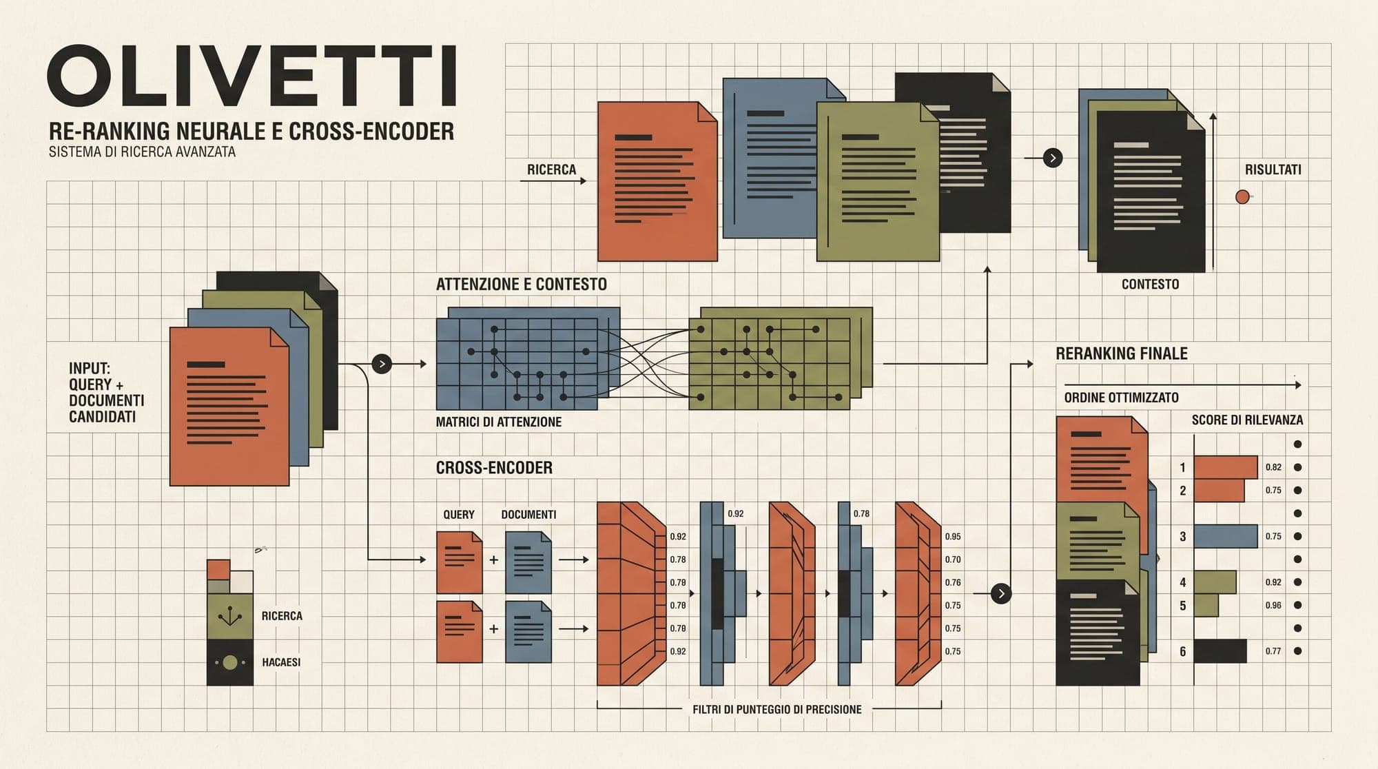
Context Reranking Engines in Production RAG: Comparing Cohere Rerank, BGE-Reranker-v2, FlashRank, and ColBERT Late Interaction

Standard Retrieval-Augmented Generation (RAG) pipelines frequently face a fundamental retrieval bottleneck: single-vector bi-encoders compress variable-length documents into a single dense embedding. While dense vector search enables high-throughput approximate nearest neighbor (ANN) retrieval across millions of documents, it discards token-level interactions. This compression creates well-documented failure modes in keyword specificity, fine-grained entity constraints, and logical negation.

Production RAG systems resolve this through a two-stage retrieval architecture: a high-recall first-stage retriever (combining BM25 lexical search and dense vector search) gathers an initial candidate set of 50 to 100 documents, followed by a high-precision second-stage reranking engine that scores and reorders candidates before context is injected into the generative model's prompt window.

This analysis evaluates four distinct reranking paradigms: full cross-encoder self-attention (Cohere Rerank 3.5 and BGE-Reranker-v2), multi-vector late interaction (ColBERTv2 and PLAID), ultra-lightweight CPU-native ONNX execution (FlashRank), and causal listwise interaction (Jina Reranker v3).

1. The Vector Compression Problem and Two-Stage Retrieval

In single-vector retrieval, both the query $q$ and document $d$ are mapped into fixed-dimensional vectors:

$$\mathbf{u} = \text{Encoder}(q), \quad \mathbf{v} = \text{Encoder}(d), \quad S(q, d) = \cos(\mathbf{u}, \mathbf{v}) = \frac{\mathbf{u} \cdot \mathbf{v}}{\|\mathbf{u}\| \|\mathbf{v}\|}$$

Because encoding occurs independently without cross-attention between $q$ and $d$, the vector representation must summarize all semantic dimensions into 768 to 3072 floating-point values.

This architectural separation creates three primary failure modes in production:

• Negation Blindness: A query asking for "open-source models excluding Apache licenses" often matches documents describing "open-source models with Apache licenses" because the shared semantic tokens overwhelm the isolated negation token during pooling.
• Lexical Dilution: When a query specifies a strict identifier, SKU, or error code, semantic embeddings often pull conceptually similar passages while missing the exact keyword match.
• Information Density Skew: Long documents contain disparate concepts. Mean pooling or CLS pooling dilutes local paragraphs containing the exact answer.

Two-stage retrieval addresses this by splitting the retrieval burden: Stage 1 optimizes for recall over the entire corpus with sub-10ms vector and keyword indices, while Stage 2 optimizes for precision over a bounded candidate window (top 50 to 100 passages) using deep token-level cross-attention.

2. Architectural Paradigms Compared

1. Bi-Encoder (Stage 1):
   Query   ---> [ Encoder ] ---> Vector Q ---\
                                              Cosine / Dot Product ---> Fast Candidate Top-K
   Doc     ---> [ Encoder ] ---> Vector D ---/

2. Cross-Encoder (Stage 2 - Full Self-Attention):
   [CLS] + Query + [SEP] + Doc ---> [ Full Transformer Layers ] ---> All-to-All Attention Matrix ---> Probability Score

3. Late Interaction (Stage 2 - ColBERT / MaxSim):
   Query   ---> [ Encoder ] ---> [ q1, q2, ..., qn ] ---\
                                                         MaxSim: Sum(Max(qi . dj)) ---> Calibrated Score
   Doc     ---> [ Encoder ] ---> [ d1, d2, ..., dm ] ---/

4. Ultra-Lite ONNX / CPU (Stage 2 - Quantized Cross-Encoder):
   [CLS] + Query + [SEP] + Doc ---> [ Quantized ONNX Runtime ] ---> Sub-15ms Score

Full Cross-Encoder Self-Attention: Cohere Rerank and BGE-Reranker-v2

In a cross-encoder, the query and candidate passage are concatenated into a unified sequence:

$$\text{Input} = [\text{CLS}] \circ q \circ [\text{SEP}] \circ d \circ [\text{SEP}]$$

The concatenated sequence is processed simultaneously through every layer of the transformer backbone.

• Attention Mechanics: Every query token attends directly to every document token across all attention heads and layers. This allows the model to capture syntactic relationships, modifier scoping, and precise entity associations.
• Computational Cost: Cross-attention complexity scales quadratically $\mathcal{O}((N + M)^2)$ with total sequence length $N + M$. Scoring 100 documents requires 100 independent forward passes of length $N + M$.
• Context Capacity: Cohere Rerank 3 and 3.5 support context lengths up to 4,096 tokens per document, specifically handling semi-structured tables, JSON objects, and code snippets. BAAI's BGE-Reranker-v2-m3 uses a 568M-parameter XLM-RoBERTa architecture supporting 512 to 1,024 tokens across multilingual corpora, while bge-reranker-v2-gemma scales to 2.5B parameters for higher precision.

Multi-Vector Late Interaction: ColBERTv2 and PLAID

ColBERTv2 (Contextualized Late Interaction over BERT) introduces a middle ground between bi-encoders and cross-encoders.

• Token-Level Encodings: Rather than pooling tokens into a single vector, ColBERT produces a sequence of low-dimensional vectors (typically 128 dimensions per token) for both query and document:

$$Q = E_Q(q) \in \mathbb{R}^{N \times 128}, \quad D = E_D(d) \in \mathbb{R}^{M \times 128}$$

• MaxSim Interaction: Document token vectors are computed offline and indexed. At query time, the system computes the inner product between each query token and all document tokens, finds the maximum match per query token, and sums these maximums:

$$S(q, d) = \sum_{i=1}^{N} \max_{j=1}^{M} \left( \mathbf{q}_i \cdot \mathbf{d}_j \right)$$

• PLAID Engine Optimization: The Performance-Optimized Late Interaction Driver (PLAID) clusters document token embeddings into centroids. By pruning unpromising passages at the centroid stage before full MaxSim calculation, PLAID reduces GPU search latency by 2.5x to 7x and CPU latency by up to 45x compared to standard ColBERTv2, achieving sub-35ms top-100 retrieval on MS MARCO.

Ultra-Lightweight ONNX Reranking: FlashRank

FlashRank is designed for environments where installing heavyweight frameworks like PyTorch or Hugging Face Transformers is impractical due to container size limits, cold-start latency, or GPU unavailability.

• Runtime Optimization: Built exclusively on ONNX Runtime, eliminating Python deep learning framework overhead and multi-gigabyte virtual environments.
• Model Footprint: Offers quantized models ranging from ~4MB (ms-marco-TinyBERT-L-2-v2) to ~34MB (ms-marco-MiniLM-L-12-v2) and ~110MB (rank-T5-flan).
• Latency Profile: Executes in 8ms to 25ms on commodity 4-core CPUs for candidate lists of 50 passages, making it suitable for edge workers, AWS Lambda functions, and local desktop applications.

Causal Listwise Interaction: Jina Reranker v3

Jina Reranker v3 and v3.5 employ what the authors define as "last-but-not-late interaction."

• Mechanism: Multiple candidate passages and the user query are packed into a single causal transformer context window. The model performs causal self-attention across candidates and extracts relevance embeddings from the final token of each passage segment.
• Structured Data Handling: Specifically optimized for tool parameters, function calling signatures, and tabular JSON documents. On the BEIR benchmark suite, Jina Reranker v3 achieves 61.94 nDCG@10, outperforming conventional cross-encoders on multi-hop fact verification tasks such as FEVER (93.95) and HotpotQA (78.56).

3. Production Tradeoffs and Performance Benchmarks

Selecting a reranking engine requires navigating explicit tradeoffs across latency budgets, infrastructure footprint, and ranking precision.

Latency Profiles Across Top-50 Candidates

• Cohere Rerank 3.5 (API): 150ms to 300ms total request latency (including 50ms to 100ms network round-trip overhead). Per Oracle Cloud Infrastructure benchmarks, request latency scales from 0.16s for 48 documents of 256 tokens to 0.73s for 48 documents of 1024 tokens.
• BGE-Reranker-v2-m3 (Dedicated L4/A10 GPU): 50ms to 120ms for 50 candidates at 512 tokens. Throughput reaches approximately 1,100 pair evaluations per second.
• PLAID ColBERTv2 (GPU): 15ms to 35ms for top-100 candidates on an A10 GPU, with minimal latency growth as document length scales due to pre-computed document token caches.
• FlashRank MiniLM-L-12 (4-Core CPU): 8ms to 25ms for 50 candidates, requiring zero GPU allocation and under 150MB of host RAM.
• Jina Reranker v3 (Dedicated GPU): 70ms to 150ms for 50 candidates, scaling with total concatenated context length.

Accuracy vs Latency Frontier

Retrieval Accuracy (NDCG@10)
    ^
    |                                   * Cohere Rerank 3.5 (NDCG: ~0.71-0.77)
    |                      * BGE-Reranker-v2-m3 (MTEB: 60.4)
    |           * PLAID ColBERTv2 (MRR@10: ~39.8)
    |
    |   * FlashRank MiniLM-L-12 (Fast CPU baseline)
    |
    +------------------------------------------------------------->
    0 ms        25 ms       50 ms       100 ms      200 ms     300 ms
                             p95 Query Latency

• High-Precision Applications (Legal discovery, compliance verification, medical literature search): Full cross-encoders (Cohere Rerank 3.5 or BGE-Reranker-v2-gemma) are mandatory. The 150ms to 300ms latency penalty is acceptable when downstream error costs are severe.
• Conversational and Voice AI (Interactive agents, sub-500ms voice turns): Total system latency budgets typically allocate at most 50ms to information retrieval. In these environments, FlashRank or PLAID ColBERTv2 fit the required time window.
• Index Storage Overhead: While cross-encoders and FlashRank compute scores on raw text returned by the primary database, ColBERT requires persisting token embeddings for every indexed passage. This increases vector storage requirements from 1.5KB per document to 15KB-30KB per document.

4. Serving Economics: API vs Dedicated GPU vs In-Process CPU

The total cost of ownership (TCO) across reranking architectures shifts dramatically based on request volume:

Managed API Model (Cohere Rerank)

• Cost Structure: Approximately $2.00 per 1,000 search queries ($0.002 per call).
• Monthly TCO at 50,000 queries/month: $100.
• Monthly TCO at 2,000,000 queries/month: $4,000.
• Operational Profile: Zero infrastructure maintenance, automatic scaling, built-in multi-aspect document handling, but bounded by external network latency and third-party data transmission policies.

Dedicated GPU Microservice (BGE-Reranker-v2 on Hugging Face TEI / vLLM)

• Cost Structure: One cloud NVIDIA L4 instance (24GB VRAM) costs approximately $0.70/hour ($504/month).
• Throughput Capacity: Capable of serving 25 to 50 reranking requests per second (equivalent to 65M to 130M monthly evaluations).
• Breakeven Threshold: Self-hosting becomes cost-effective once query volume exceeds 250,000 requests per month ($500 API cost threshold).
• Operational Profile: Requires Kubernetes or container cluster management, health monitoring, and autoscaling policies.

In-Process CPU Reranker (FlashRank / ONNX)

• Cost Structure: $0 incremental infrastructure cost. Runs directly inside existing application containers or serverless runtimes (AWS Lambda, Google Cloud Run).
• Operational Profile: Minimal operational surface, zero GPU dependency, sub-second container cold starts, and deterministic memory consumption (< 200MB).

5. Implementation Pattern: Two-Stage Production Pipeline

Below is an implementation of a two-stage retrieval pipeline using hybrid candidate generation, dynamic score thresholding, and fallback logic:

from dataclasses import dataclass
from typing import List, Dict, Any, Optional
import numpy as np
from flashrank import Ranker, RerankRequest

@dataclass
class RetrievedDocument:
    id: str
    text: str
    stage1_score: float
    rerank_score: float = 0.0

class ProductionTwoStageRetriever:
    def __init__(
        self,
        model_name: str = "ms-marco-MiniLM-L-12-v2",
        cache_dir: str = "/tmp/flashrank_models",
        max_context_length: int = 512,
    ):
        # Initialize lightweight ONNX reranking engine
        self.ranker = Ranker(
            model_name=model_name,
            cache_dir=cache_dir,
            max_length=max_context_length,
        )

    def rerank(
        self,
        query: str,
        candidates: List[Dict[str, Any]],
        top_k: int = 5,
        score_threshold: float = 0.30,
    ) -> List[RetrievedDocument]:
        """
        Reranks first-stage candidate passages and applies dynamic score thresholding.
        """
        if not candidates:
            return []

        # Format candidate passages for the reranker
        passages = [
            {"id": str(item["id"]), "text": item["text"]}
            for item in candidates
        ]

        # Execute ONNX cross-encoder inference
        request = RerankRequest(query=query, passages=passages)
        scored_results = self.ranker.rerank(request)

        # Apply score calibration and extract top-k
        final_documents: List[RetrievedDocument] = []
        for result in scored_results:
            score = float(result.get("score", 0.0))
            if score >= score_threshold:
                # Map back stage 1 score for observability
                original_score = next(
                    (float(c.get("score", 0.0)) for c in candidates if str(c["id"]) == str(result["id"])),
                    0.0
                )
                final_documents.append(
                    RetrievedDocument(
                        id=result["id"],
                        text=result["text"],
                        stage1_score=original_score,
                        rerank_score=score,
                    )
                )

            if len(final_documents) >= top_k:
                break

        # Fallback: if no document meets the threshold, return top-1 candidate to prevent empty prompt context
        if not final_documents and scored_results:
            top_result = scored_results[0]
            final_documents.append(
                RetrievedDocument(
                    id=top_result["id"],
                    text=top_result["text"],
                    stage1_score=0.0,
                    rerank_score=float(top_result.get("score", 0.0)),
                )
            )

        return final_documents

6. Key Engineering Rules for Production Deployment

1. Passage Truncation Before Cross-Attention: Over 90% of cross-encoder relevance discriminant information sits within the first 256 to 384 tokens of a chunk. Truncating candidate passages to 384 tokens before scoring cuts quadratic attention compute without meaningful loss in NDCG@10.
2. Context Window Token Reduction: Feeding 50 raw retrieved chunks into a frontier LLM costs thousands of input tokens per request. Reranking and filtering down to the top 3 or top 5 high-relevance chunks reduces LLM prompt tokens by 75% to 90%, speeding up generative time-to-first-token (TTFT) and lowering overall inference costs.
3. Dynamic Thresholding Over Fixed Top-K: Passing a fixed number of chunks (e.g., always exactly 5) forces low-scoring irrelevant noise into the context when only 1 or 2 passages are relevant. Enforcing a calibrated score cutoff ensures the generative model receives only verified evidence.

Sources

• Cohere Rerank 3 Announcement and Technical Specifications
• Cohere Rerank 3.5 Latency and Throughput Benchmarks - Oracle Cloud Infrastructure
• BAAI BGE Reranker Documentation and Architecture Specifications
• PLAID: An Efficient Engine for Late Interaction Retrieval (Santhanam et al., Stanford University / arXiv)
• FlashRank: Lightweight ONNX-Powered Reranking Engine (Prithiviraj Damodaran)
• jina-reranker-v3: Last but Not Late Interaction for Document Reranking (Jina AI / arXiv)
• Jina Reranker v3.5 for Legal, Medical, and Structured Search - Elasticsearch Labs
• RAG Reranking: Improving Retrieval Quality with Cross-Encoders - BigData Boutique