Activation Checkpointing in Large Language Models: How Selective Recomputation Eliminates Memory Bottlenecks

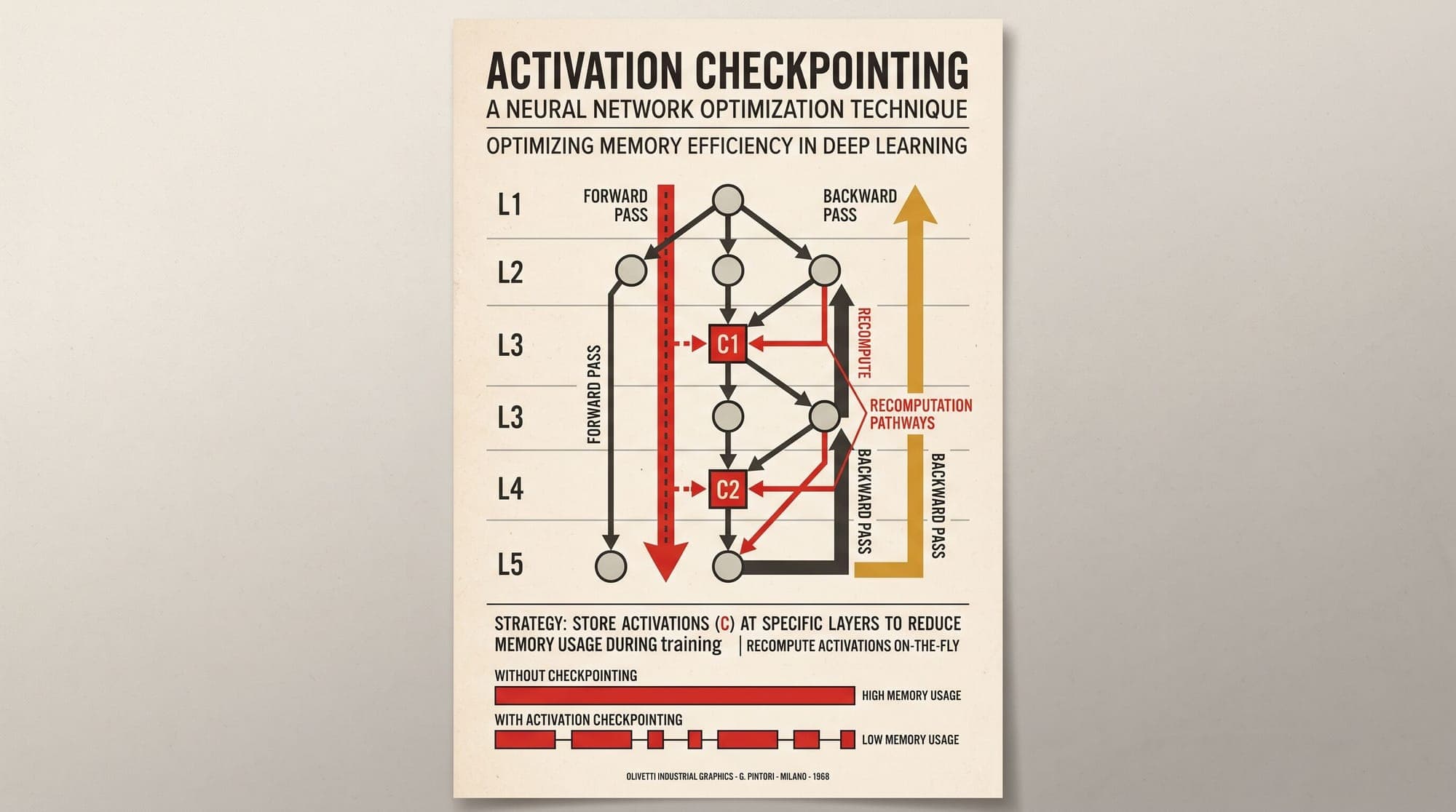
Large language model pre-training and fine-tuning are fundamentally constrained by GPU memory (VRAM). While distributed techniques such as Fully Sharded Data Parallel (FSDP), ZeRO, and Tensor Parallelism successfully shard model parameters, optimizer states, and gradients across hundreds or thousands of GPUs, activation memory presents a distinct scaling bottleneck.

During the forward pass of a transformer model, intermediate tensor outputs must be preserved in GPU memory so that backpropagation can compute exact analytical gradients using the chain rule. As sequence lengths extend from 2,048 tokens to 32,768, 128,000, and beyond, activation memory scales with sequence length and batch size, rapidly outstripping the memory required to store the model weights themselves.

Activation checkpointing, originally introduced as gradient checkpointing, resolves this memory wall by trading a modest amount of extra computation for substantial memory reductions. Modern LLM training systems have evolved this technique from coarse layer-level recomputation to fine-grained selective activation recomputation, enabling multi-billion parameter models with massive context windows to train without exhausting device memory.

The Origin of the Activation Memory Bottleneck

To understand why activation memory grows so rapidly, consider the mechanics of reverse-mode automatic differentiation in deep neural networks. For any parameterized layer performing the forward transformation $y = f(x, W)$, the backward pass requires computing gradients with respect to both the parameters $W$ and the inputs $x$:

$$\frac{\partial \mathcal{L}}{\partial W} = \frac{\partial \mathcal{L}}{\partial y} \cdot \frac{\partial y}{\partial W} = \frac{\partial \mathcal{L}}{\partial y} \cdot x^T$$

$$\frac{\partial \mathcal{L}}{\partial x} = W^T \cdot \frac{\partial \mathcal{L}}{\partial y}$$

Calculating the parameter gradient $\frac{\partial \mathcal{L}}{\partial W}$ requires access to the forward activation tensor $x$. In standard backpropagation, the execution engine stores every intermediate activation tensor generated during the forward pass in High Bandwidth Memory (HBM) until the backward pass traverses back to that layer.

In a deep transformer with $L$ layers, hidden dimension $h$, sequence length $s$, and micro-batch size $b$, the number of stored tensors scales linearly with depth and context length, alongside quadratic terms introduced by standard multi-head self-attention. For long-context models, storing every activation tensor leads to Out-Of-Memory (OOM) faults before training can complete a single optimization step.

Classic Gradient Checkpointing: The Sublinear Trade-off

The mathematical foundation of activation recomputation was formalized by Tianqi Chen et al. in their 2016 paper, Training Deep Nets with Sublinear Memory Cost.

Chen et al. formulated memory optimization as a graph traversal problem. Instead of caching all intermediate activation tensors throughout an $N$-node computation graph:

1. Checkpoints: The model retains forward activations only at specific designated checkpoint nodes (for instance, the input tensor to every $k$-th layer).
2. Discards: All intermediate activation tensors between checkpoint boundaries are immediately freed from GPU memory during the forward pass.
3. Recomputation: During the backward pass, when gradients are needed for a segment between checkpoints, the system executes a localized forward pass starting from the stored checkpoint tensor to regenerate the discarded activations just in time.

By selecting an optimal checkpoint spacing of $k = \sqrt{N}$, the total memory required to store activations drops from $O(N)$ to $O(\sqrt{N})$.

The Compute Overhead of Full Recomputation

The memory reduction comes at the cost of additional compute. In standard backpropagation:

• The forward pass performs approximately $2P$ floating-point operations (FLOPs) per token, where $P$ is the parameter count.
• The backward pass performs approximately $4P$ FLOPs per token (computing gradients for weights and inputs).
• Total training FLOPs per step equal $6P$.

Under full layer-level activation checkpointing, every transformer layer executes a second forward pass during backpropagation, adding $2P$ FLOPs. This increases total compute from $6P$ to $8P$ FLOPs, representing an exact 33.3% computational overhead.

Transformer Layer Activation Anatomy

To optimize activation management beyond coarse full-layer checkpointing, Korthikanti et al. (2022) in Reducing Activation Recomputation in Large Transformer Models derived an exact analytical breakdown of activation memory inside a standard transformer layer.

For a transformer layer operating in 16-bit precision (2 bytes per element) with hidden size $h$, sequence length $s$, micro-batch size $b$, and $a$ attention heads, the memory required to store activations without checkpointing comprises:

Component Breakdown (per Transformer Layer, 16-bit precision):
--------------------------------------------------------------------------------
1. Pre-Attention Normalization (RMSNorm/LayerNorm):    4 * s * b * h bytes
2. Self-Attention QKV Projections:                    6 * s * b * h bytes
3. Attention Core Matrices (Q * K^T):                 2 * s^2 * b * a bytes
4. Softmax Output Probabilities:                      2 * s^2 * b * a bytes
5. Attention Dropout Mask & Output:                   3 * s^2 * b * a bytes
6. Attention Value Context (Attention * V):           2 * s * b * h bytes
7. Attention Output Projection:                       2 * s * b * h bytes
8. Post-Attention Normalization:                      4 * s * b * h bytes
9. Feed-Forward MLP Up-Projection / Gating:           8 * s * b * h bytes
10. MLP Activation Function (GeLU / SwiGLU):          8 * s * b * h bytes
11. MLP Down-Projection:                              2 * s * b * h bytes
12. Residual Connection Dropouts:                     4 * s * b * h bytes
--------------------------------------------------------------------------------
Total Memory per Layer without Checkpointing:
  sbh * (34 + 5 * (a * s / h)) bytes

This equation reveals a critical asymmetry in transformer memory consumption:

• Linear Terms ($34sbh$): Generated by General Matrix Multiply (GEMM) operations across projections and feed-forward networks, scaling linearly with sequence length $s$.
• Quadratic Attention Terms ($5 s^2 b a$): Generated by intermediate attention score matrices, softmax distributions, and dropout masks, scaling quadratically with sequence length $s$.

When sequence length $s$ is large relative to hidden dimension $h$, the quadratic term $5 \frac{a s}{h}$ dominates total memory consumption.

Selective Activation Recomputation

The central insight of selective activation recomputation is that memory consumption and computational intensity are inversely distributed across transformer operations:

• GEMM Projections: Linear projections (QKV, Attention Output, MLP Up/Down) account for over 98% of the mathematical FLOPs in a transformer layer, but produce relatively compact activation tensors of size $s \times b \times h$.
• Attention Operations: Softmax, dropout, and matrix multiplications between queries, keys, and values account for less than 2% of total layer FLOPs, but generate the massive $s \times s$ attention matrices that consume the majority of activation memory.

Instead of discarding and recomputing the entire layer (which forces expensive GEMMs to run twice), selective activation recomputation retains the inputs to all linear layers while discarding only the activation tensors of the memory-heavy, FLOP-light attention operators.

Activation Recomputation Strategies Comparison:
--------------------------------------------------------------------------------
Strategy: Full Recomputation
- Stored at Forward: Only input tensor x_l to the transformer layer
- Activation Memory per Layer: 2 * s * b * h bytes
- Compute Overhead: ~33.3% additional FLOPs
- Bottleneck: Redundant GEMM computations during backward pass

Strategy: Selective Recomputation
- Stored at Forward: Inputs to GEMMs (Q, K, V projections and MLP layers)
- Discarded & Recomputed: QK^T matrix, Softmax probabilities, Dropout masks
- Activation Memory per Layer: 34 * s * b * h bytes
- Compute Overhead: ~2.0% to 4.0% additional FLOPs
- Advantage: Eliminates quadratic O(s^2) memory scaling with negligible FLOP cost

Strategy: No Checkpointing
- Stored at Forward: All intermediate tensors, masks, and attention scores
- Activation Memory per Layer: sbh * (34 + 5 * (a * s / h)) bytes
- Compute Overhead: 0%
- Limitation: Severe VRAM limits, unviable for long sequences

By discarding only the attention matrices and recomputing them on the fly from the cached Q, K, and V tensors during backpropagation, selective recomputation eliminates the quadratic memory term while keeping the compute overhead below 4%.

FlashAttention as Built-in Selective Recomputation

The principles of selective activation recomputation reached their logical hardware-aware culmination with Dao et al.'s FlashAttention (2022) and FlashAttention-2 (2023).

Standard PyTorch implementations of attention write intermediate $s \times s$ matrices to GPU High Bandwidth Memory (HBM) and read them back during softmax and dropout. FlashAttention fuses the entire attention block into a single GPU kernel using SRAM tiling and online softmax scaling.

Crucially, FlashAttention integrates selective activation recomputation by design:

1. Forward Pass: The forward kernel computes attention outputs without ever materializing or writing the $s \times s$ attention score matrix or softmax probabilities to HBM. It stores only the final output tensor and small per-token softmax normalization statistics (the row-wise maximum $m$ and sum of exponentials $l$).
2. Backward Pass: When computing gradients with respect to Q, K, and V, the backward kernel loads blocks of Q, K, and V from HBM into fast on-chip SRAM, recomputes the corresponding tile of the attention matrix on the fly using the stored normalization statistics, and immediately accumulates the weight gradients.

Because SRAM bandwidth is an order of magnitude faster than HBM bandwidth, recomputing attention scores directly in SRAM during backpropagation is faster than reading cached attention matrices from global GPU memory.

Implementation Details in PyTorch and Distributed Frameworks

Modern distributed training frameworks like Megatron-Core, DeepSpeed, and PyTorch implement activation checkpointing through customizable policies.

PyTorch torch.utils.checkpoint

PyTorch provides activation checkpointing through torch.utils.checkpoint.checkpoint. Modern implementations prefer use_reentrant=False, which relies on standard autograd engine hooks rather than creating a separate nested autograd graph:

import torch
import torch.nn as nn
from torch.utils.checkpoint import checkpoint

class TransformerBlock(nn.Module):
    def __init__(self, d_model, n_heads):
        super().__init__()
        self.attn = nn.MultiheadAttention(d_model, n_heads)
        self.mlp = nn.Sequential(
            nn.Linear(d_model, 4 * d_model),
            nn.GELU(),
            nn.Linear(4 * d_model, d_model)
        )
        self.norm1 = nn.LayerNorm(d_model)
        self.norm2 = nn.LayerNorm(d_model)

    def forward(self, x):
        # Attention block with residual
        norm_x = self.norm1(x)
        attn_out, _ = self.attn(norm_x, norm_x, norm_x)
        x = x + attn_out
        
        # MLP block with residual
        norm_x = self.norm2(x)
        mlp_out = self.mlp(norm_x)
        x = x + mlp_out
        return x

class CheckpointedTransformer(nn.Module):
    def __init__(self, num_layers, d_model, n_heads):
        super().__init__()
        self.layers = nn.ModuleList([
            TransformerBlock(d_model, n_heads) for _ in range(num_layers)
        ])

    def forward(self, x):
        for layer in self.layers:
            # Checkpoint the entire block boundary
            x = checkpoint(layer, x, use_reentrant=False)
        return x

Distributed Interaction: Sequence Parallelism and FSDP

When training frontier models across clusters:

1. Combining with Sequence Parallelism (Megatron-SP): In standard Tensor Parallelism, LayerNorm and Dropout activations are replicated across all GPUs within the tensor parallel group. Megatron-SP shards these activations across the sequence dimension. When combined with selective recomputation, activation memory per device scales as:

$$\text{Memory}_{\text{per-GPU}} = \frac{s \cdot b \cdot h}{t} \cdot 34$$

where $t$ is the tensor parallel degree.

1. Interleaving with Fully Sharded Data Parallel (FSDP / ZeRO-3): When activation checkpointing is used with FSDP, discarded layers do not retain forward activations. During the backward recomputation pass, FSDP must re-fetch sharded model parameters via All-Gather before recomputing forward activations, introducing a communication-compute overlap consideration that distributed engines schedule to avoid GPU stalling.

Practical Decision Matrix for LLM Training

Selecting the optimal activation checkpointing configuration depends on model architecture, sequence length, and hardware constraints:

• Short Contexts (s <= 2,048 tokens, small batch): When model parameters fit comfortably in VRAM alongside activations, disable activation checkpointing entirely to achieve maximum training throughput (0% FLOP overhead).
• Standard Pre-Training (s = 4,096 to 8,192 tokens): Deploy Selective Activation Recomputation combined with FlashAttention. This eliminates memory bottlenecks from attention score matrices while incurring less than 3% FLOP overhead, allowing maximum micro-batch sizes without OOMs.
• Ultra Long Contexts (s >= 32,768 tokens) or Memory-Constrained Fine-Tuning: Deploy Full Layer Checkpointing (or selective checkpointing coupled with Sequence Parallelism and CPU offloading). While full checkpointing incurs a 33% compute penalty, it reduces per-layer activation footprint to a single boundary tensor, making massive context windows physically trainable on available hardware.

Sources

• Tianqi Chen, Bing Xu, Chiyuan Zhang, Carlos Guestrin (2016). Training Deep Nets with Sublinear Memory Cost. arXiv:1604.06174
• Vijay Anand Korthikanti, Jared Casper, Sangkug Lym, Lawrence C. McAfee, Michael Andersch, Mohammad Shoeybi, Bryan Catanzaro (2022). Reducing Activation Recomputation in Large Transformer Models. arXiv:2205.05198
• Tri Dao, Daniel Y. Fu, Stefano Ermon, Atri Rudra, Christopher Ré (2022). FlashAttention: Fast and Memory-Efficient Exact Attention with IO-Awareness. arXiv:2205.14135
• Tri Dao (2023). FlashAttention-2: Faster Attention with Better Parallelism and Work Partitioning. arXiv:2307.08691
• Mohammad Shoeybi, Mostofa Patwary, Raul Puri, Patrick LeGresley, Jared Casper, Bryan Catanzaro (2019). Megatron-LM: Training Multi-Billion Parameter Language Models Using Model Parallelism. arXiv:1909.08053
• PyTorch Documentation: torch.utils.checkpoint